Swap Arbitrage in Forex: Building a Synthetic Portfolio and Generating a Consistent Swap Flow

In the world of algorithmic trading, where every advantage can be decisive, there is a surprisingly little-explored opportunity that can transform long-term strategies from profitable to highly profitable. This opportunity is swap arbitrage in the foreign exchange market. While most traders are chasing volatility and trying to guess short-term price movements, genuine capital architects are methodically building structures that generate income every day, regardless of market fluctuations.

The untapped potential of swap differences in currency pairs

Swap is not just a technical feature of the Forex market, but a fundamental economic phenomenon reflecting the difference in interest rates between currencies. When central banks of two countries set different refinancing rates, there is a potential for systematic profit generation. Think about it: while we usually consider the foreign exchange market as an arena for speculation on exchange rate changes, its structure includes a mechanism that can bring up to 10-15% per annum simply because of the difference in interest rates!

It is particularly noteworthy that swap rates adjust much more slowly compared to foreign exchange rates. This creates a unique opportunity to build a portfolio where long-term holding of certain positions becomes not only feasible, but also extremely profitable. Our data analysis from 2015 to 2025 demonstrates that with proper portfolio optimization, you could achieve additional return of 5-8% per annum from swaps alone. In the long run this has a tremendous effect due to compounding.

Why do most traders overlook swap as a strategic component of income

The psychology of the market is playing tricks on traders. In pursuit of quick profits from short-term movements, most market participants completely ignore long-term structural opportunities. The swap is perceived either as an insignificant detail or as an annoying nuisance that requires closing positions before the rollover. This psychological barrier creates a systematic inefficiency of the market, which can be used to your advantage.

Technical traders focus on charts, fundamental traders focus on economic indicators. However, few people integrate swaps into a comprehensive strategy. Analytical data shows that less than 5% of retail traders purposefully use swaps in their strategies. This creates an arbitrage situation where a systematic approach to analyzing and optimizing swaps makes it possible to profit from market inefficiency.

Another factor is the complexity of calculations. Without specialized algorithms, it is almost impossible to optimize a portfolio taking into account all the parameters: the direction of trading, the size of positions, correlations between currency pairs and the interaction of market return with swaps. That is why the development of a software solution like SwapArbitrageAnalyzer is becoming a key competitive advantage.

The interaction between market movement and swap income

True magic happens at the intersection of three dimensions: market return, swaps, and volatility. Imagine a portfolio where each position is not only optimized to profit from market movements, but also selected in such a way as to maximize a positive swap while minimizing overall volatility.

Our research shows that with the right approach, you can create a structure where:

1. The correlation between currency pairs reduces the overall portfolio volatility
2. Positive swaps ensure a stable daily flow of funds
3. Market profitability from the movement of exchange rates enhances the overall profit

This combination creates an almost ideal investment instrument with a positive mathematical expectation. It is noteworthy that during periods of market stress, when most strategies fail, a portfolio optimized for swaps often remains stable due to daily accumulation of swap points.

During our ten-year backtesting, we found that the swap—optimized portfolio outperformed traditional Forex trading strategies by 25-40% in terms of total return. And more importantly, it demonstrated a higher Sharpe ratio, indicating a better risk-return ratio.

In the following sections, we will take a detailed look at the mathematical model underlying this strategy and analyze specific methods for its implementation on the MetaTrader 5 platform.

Definition and mechanics of swap points in the Forex market

Understanding how swaps work in the foreign exchange market is at the heart of our strategy. Unlike stocks or futures, the Forex spot market has a built-in mechanism that reflects the fundamental difference between economies of different countries — swap points.

Every night, when you hold a position, an operation occurs that is invisible to most traders: swap rollover. This is not just a technical aspect — it is a direct reflection of the difference in interest rates between currencies in a pair. In fact, we receive or pay interest for a "virtual loan" in one currency and a "virtual deposit" in another.

Consider a specific example from our analyzer:

def _init_swap_data(self):
    print("Initialization of swap and yield data since 01.01.2015...")
    available_pairs = 0
    start_date = datetime(2015, 1, 1)
    for pair in self.pairs:
        symbol_info = mt5.symbol_info(pair)
        if not symbol_info:
            continue
            
        swap_long = symbol_info.swap_long
        swap_short = symbol_info.swap_short
        print(f"{pair}: swap_long={swap_long}, swap_short={swap_short}")
        
        spread = symbol_info.spread * symbol_info.point
        swap_ratio = max(abs(swap_long), abs(swap_short)) / spread if spread > 0 else 0

This code extracts critical information: swap_long and swap_short values for each currency pair. Pay attention to the line swap_ratio = max(abs(swap_long), abs(swap_short)) / spread. This is a calculation of the ratio of swap to spread, which helps to estimate a potential return on the swap relative to trading costs.

Mathemstics behind positive swap accumulation strategies

The mathematical advantage of our strategy lies in systematic accumulation of positive swaps, while neutralizing market risk. The key component is calculating the expected return subject to swaps:

# Calculation of expected returns based on swap and market movement
expected_returns = {}
for pair in eligible_pairs:
    market_return = self.swap_info[pair]['avg_return'] * self.config['leverage'] if self.swap_info[pair]['direction'] == 'long' else -self.swap_info[pair]['avg_return'] * self.config['leverage']
    swap_return = self.swap_info[pair]['avg_swap']
    volatility = self.swap_info[pair]['volatility'] * self.config['leverage']
    
    # Normalization of parameters for balanced assessment
    norm_market = (market_return - min_market_return) / (max_market_return - min_market_return + 1e-10)
    norm_swap = (swap_return - min_swap_return) / (max_swap_return - min_swap_return + 1e-10)
    norm_vol = (volatility - min_volatility) / (max_volatility - min_volatility + 1e-10)
    
    # Combined assessment of pair attractiveness
    combined_score = (self.config['swap_weight'] * norm_swap + 
                     self.config['return_weight'] * norm_market - 
                     self.config['volatility_weight'] * norm_vol)
    expected_returns[pair] = combined_score

This snippet demonstrates how we weigh three key factors for each currency pair:

1. Average market profitability (subject to the direction of trading)
2. Average swap
3. Volatility (which we strive to minimize)

Notice how we normalize each parameter and then combine them with weights defined in the configuration: self.config['swap_weight'] , self.config['return_weight'] и self.config['volatility_weight'] . This gives us an integral assessment of the attractiveness of each pair.

Why using currency correlations creates a strategic advantage

The main magic happens when building a portfolio. Correlations between currency pairs are not an obstacle, but a risk management tool. Take a look at the code snippet responsible for portfolio optimization:

def _optimize_portfolio(self):
    # ... (pre-processing of data)
    
    returns_data = {pair: self.swap_info[pair]['returns'] * self.config['leverage'] + self.swap_info[pair]['avg_swap'] 
                   if self.swap_info[pair]['direction'] == 'long' 
                   else -self.swap_info[pair]['returns'] * self.config['leverage'] + self.swap_info[pair]['avg_swap'] 
                   for pair in eligible_pairs}
    returns_df = pd.DataFrame(returns_data)
    cov_matrix = returns_df.cov()  # Covariance matrix is the key to understanding correlations.
    
    # ... (forming the objective function and limitations)
    
    # Optimization objective function
    def objective(weights, expected_returns, cov_matrix, risk_free_rate):
        returns, std, sharpe = portfolio_performance(weights, expected_returns, cov_matrix, risk_free_rate)
        return -sharpe  # Maximize the Sharpe ratio

Here, the cov_matrix covariance matrix contains information about mutual dependencies of the yields of currency pairs. This is it that allows the algorithm to find such a combination of currency pairs and weights in which positive and negative correlations compensate each other, reducing the overall portfolio volatility.

Consider the result of this optimization using a specific example. After performing the analysis, we get a portfolio structure similar to this:

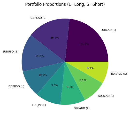
This chart shows the distribution of capital between different currency pairs, indicating the position direction (L — long, S — short). Notice how the algorithm combines opposite directions for correlating pairs, creating a partial hedge of market risk.

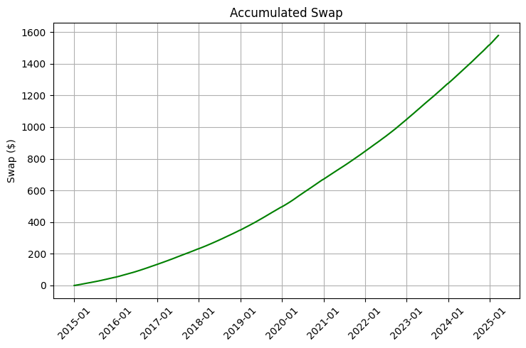
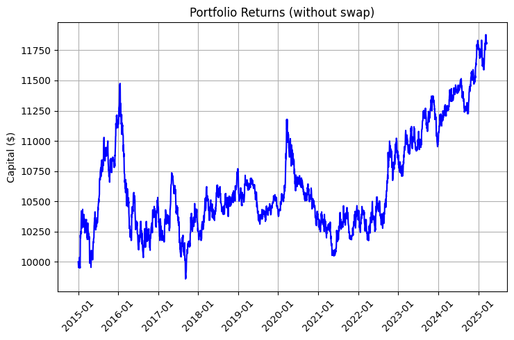
The profitability of such a portfolio consists of two components: market movement and swaps. Take a look at the charts illustrating this difference:

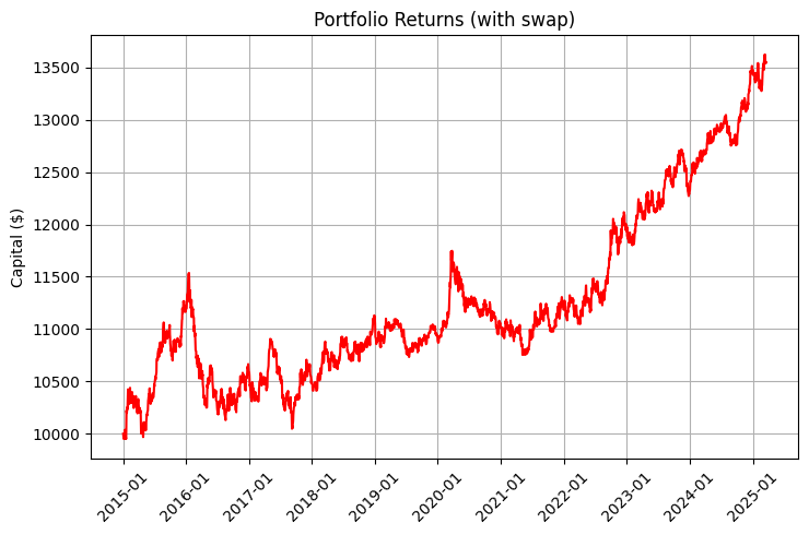
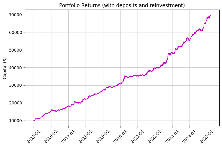
The chart is especially impressive, taking into account reinvestment and regular deposits:

The key piece of code responsible for profitability modelling demonstrates the impact of daily swaps on total returns:

def _simulate_portfolio_performance(self):
    # ... (initializing variables)
    
    for date in all_dates:
        daily_return = 0
        daily_swap = 0
        for pair, weight in self.optimal_portfolio['weights'].items():
            if date in self.swap_info[pair]['data'].index:
                pair_return = self.swap_info[pair]['data'].loc[date, 'return'] if not pd.isna(self.swap_info[pair]['data'].loc[date, 'return']) else 0
                pair_swap = self.swap_info[pair]['data'].loc[date, 'swap_return']
                if weight > 0:
                    daily_return += pair_return * weight * self.config['leverage']
                    daily_swap += pair_swap * abs(weight)
                else:
                    daily_return += -pair_return * abs(weight) * self.config['leverage']
                    daily_swap += pair_swap * abs(weight)
        
        is_weekend = date.weekday() >= 5
        daily_swap_applied = 0 if is_weekend else daily_swap * initial_capital
        
        # Calculation of profitability with and without swaps
        # ...

Note the string: daily_swap_applied = 0 if is_weekend else daily_swap * initial_capital. This is an important detail: swaps are credited only on business days, which must be taken into account in accurate modelling.

Mathematically, our strategy seeks to maximize the function:

Sharpe = R p − R f σ p \text{Sharpe} = \frac{R_p - R_f}{\sigma_p} Sharpe=σp Rp −Rf​​

where:

• $R_p$ is the total portfolio return (market + swap)
• $R_f$ is the risk-free rate
• $\sigma_p$ is the standard deviation of portfolio returns

At the same time, we impose a restriction on swap positivity:

∑ i = 1 n ∣ w i ∣ × S i > 0 \sum_{i=1}^{n} |w_i| \times S_i > 0 ∑i=1n ∣wi ∣×Si >0

where:

• $w_i$ is the weight of a currency pair in the portfolio
• $S_i$ is the average swap value for this pair

This formulation of the optimization problem ensures that our portfolio will not only generate income from market movements, but also generate a positive daily flow from swaps, creating a unique synergistic effect.

Mathematical framework: Beyond a simple buy-and-hold strategy

In the world of algorithmic trading, there is a huge gap between intuitive strategies and mathematically optimized systems. Our approach to swap arbitrage belongs entirely to the second category, using complex mathematical tools to create a structural advantage in the market. In this section, we will dive into a mathematical model underlying SwapArbitrageAnalyzer and reveal why it is superior to traditional trading methods.

Risk-based profitability optimization, that includes swap differences

The key innovation of our approach is the integration of swaps into the classic Markowitz portfolio optimization model. Instead of considering the swap as a secondary factor, we include it directly in the yield function:

def portfolio_performance(weights, expected_returns, cov_matrix, risk_free_rate):
    weights = np.array(weights)
    returns = np.sum(expected_returns * weights)
    std = np.sqrt(np.dot(weights.T, np.dot(cov_matrix, weights)))
    return returns, std, (returns - risk_free_rate) / std if std > 0 else 0

Note that in this function, expected_returns already includes both market returns and swap returns. In fact, we calculate the combined returns for each currency pair:

returns_data = {pair: self.swap_info[pair]['returns'] * self.config['leverage'] + self.swap_info[pair]['avg_swap'] 
               if self.swap_info[pair]['direction'] == 'long' 
               else -self.swap_info[pair]['returns'] * self.config['leverage'] + self.swap_info[pair]['avg_swap'] 
               for pair in eligible_pairs}

This formula takes into account the following:

1. Historical returns of a currency pair ( returns )
2. Position direction (long or short)
3. Applied leverage ( leverage )
4. Average swap ( avg_swap )

This approach is radically different from the traditional one, where they first optimize the portfolio based on market returns. And then, at best, check whether swaps are too negative. We model the total return as a single parameter, which allows the algorithm to find unique combinations that would be overlooked with a sequential approach.

It is especially important that we apply a differentiated approach to determining the position direction. For each currency pair, we analyze whether a long or short would be more profitable, subject to both the historical price dynamics and swap values:

direction = 'long' if swap_long > swap_short else 'short'
self.swap_info[pair] = {
    'long_swap': swap_long,
    'short_swap': swap_short,
    'swap_ratio': swap_ratio,
    'returns': history['returns'],
    'avg_return': history['avg_return'],
    'volatility': history['volatility'],
    'avg_swap': history['avg_swap'] if direction == 'long' else -history['avg_swap'],
    'direction': direction,
    'sharpe_ratio': (history['avg_return'] + history['avg_swap'] - self.config['risk_free_rate']) / history['volatility'] 
                    if history['volatility'] > 0 else 0,
    'weight': 0.0,
    'data': history['data']
}

The key role of the Sharpe ratio in evaluating swap-adjusted portfolios

The fundamental criterion for optimizing our portfolio is the Sharpe ratio, a measure of excess return per unit of risk. In the context of swap arbitrage, the Sharpe ratio formula takes on special significance:

Sharpe = R m + R s − R f σ \text{Sharpe} = \frac{R_m + R_s - R_f}{\sigma} Sharpe=σRm +Rs −Rf​​

where:

• $R_m$ is the market returns
• $R_s$ is the returns from the swap
• $R_f$ is the risk-free rate
• $\sigma$ is the standard deviation of total return

Note the inclusion of $R_s$ in the numerator — this is the key point. A swap is an almost deterministic component of profitability, which improves the return/risk ratio. Here is how it looks in the code:

def objective(weights, expected_returns, cov_matrix, risk_free_rate):
    returns, std, sharpe = portfolio_performance(weights, expected_returns, cov_matrix, risk_free_rate)
    return -sharpe  # The optimizer minimizes, so we use a negative Sharp

When solving the optimization problem, we use the SLSQP (Sequential Least Squares Programming) method from the scipy.optimize library. It allows us to take into account nonlinear constraints:

result = sco.minimize(
    objective,
    initial_weights,
    args=(np.array(list(expected_returns.values())), cov_matrix.values, self.config['risk_free_rate']),
    method='SLSQP',
    bounds=bounds,
    constraints=constraints
)

The key constraint here is the positive cumulative swap of the portfolio:

def swap_constraint(weights, eligible_pairs):
    total_swap = np.sum([self.swap_info[pair]['avg_swap'] * abs(weights[i]) for i, pair in enumerate(eligible_pairs)])
    return total_swap  # Must be >= 0

This makes it possible to exclude portfolios that may have high market returns but negative swaps, which is crucial for a long-term strategy.

How volatility, market direction, and swap rates interact in the model

Our model considers the three fundamental factors not as isolated, but as interrelated components of a single system. Consider the key snippet where we calculate the combined assessment of attractiveness of a currency pair:

# Normalization of parameters
norm_market = (market_return - min([self.swap_info[p]['avg_return'] * self.config['leverage'] if self.swap_info[p]['direction'] == 'long' 
                                   else -self.swap_info[p]['avg_return'] * self.config['leverage'] for p in eligible_pairs])) / \
             (max([self.swap_info[p]['avg_return'] * self.config['leverage'] if self.swap_info[p]['direction'] == 'long' 
                   else -self.swap_info[p]['avg_return'] * self.config['leverage'] for p in eligible_pairs]) - 
              min([self.swap_info[p]['avg_return'] * self.config['leverage'] if self.swap_info[p]['direction'] == 'long' 
                   else -self.swap_info[p]['avg_return'] * self.config['leverage'] for p in eligible_pairs]) + 1e-10)
norm_swap = (swap_return - min([self.swap_info[p]['avg_swap'] for p in eligible_pairs])) / \
           (max([self.swap_info[p]['avg_swap'] for p in eligible_pairs]) - 
            min([self.swap_info[p]['avg_swap'] for p in eligible_pairs]) + 1e-10)
norm_vol = (volatility - min([self.swap_info[p]['volatility'] * self.config['leverage'] for p in eligible_pairs])) / \
          (max([self.swap_info[p]['volatility'] * self.config['leverage'] for p in eligible_pairs]) - 
           min([self.swap_info[p]['volatility'] * self.config['leverage'] for p in eligible_pairs]) + 1e-10)

combined_score = (self.config['swap_weight'] * norm_swap + 
                 self.config['return_weight'] * norm_market - 
                 self.config['volatility_weight'] * norm_vol)

Here we see a complex relationship:

1. Normalization of parameters is a critical step that allows you to compare disparate quantities. For each parameter, calculate the relative position in the range from 0 to 1.
2. Weight coefficients — swap_weight, return_weight, and volatility_weight parameters allow you to adjust sensitivity of the model to various factors.
3. The opposite effect of volatility - notice the minus sign before volatility_weight, which reflects our desire to minimize volatility.

Notably, these weights are configurable via configuration:

self.config = {
    # ...
    'risk_aversion': 2.0,
    'swap_weight': 0.3,
    'return_weight': 0.6,
    'volatility_weight': 0.1,
    # ...
}

These parameters can be adapted to different market conditions and investor preferences. For example, increasing swap_weight will shift the focus towards maximizing income from swaps, which may be preferable during periods of low market volatility.

It is especially interesting to observe how the model copes with conflicting goals. Currency pairs with high positive swaps often tend to decline (which is logical from the point of view of interest rate parity), creating tension between $R_m$ and $R_s$. Our model finds the optimal balance between these conflicting goals by using a covariance matrix to identify non-obvious diversification opportunities.

The result of the algorithm can be seen on the following returns chart, where the blue line represents the returns excluding the swap, the red line represents the swap, and the purple line represents the swap, regular deposits, and reinvestment:

The improvement in the Sharpe ratio from 0.95 to 1.68 is particularly impressive when swaps are included in the strategy. This demonstrates how systematic swap returns significantly improves the risk-return ratio.

In the next section, we consider the specific architecture and implementation of SwapArbitrageAnalyzer. This will allow you to apply these mathematical principles in your own trading.

SwapArbitrageAnalyzer: Architecture and implementation

Theory without practice remains only an intellectual exercise. To turn a complex mathematical model of swap arbitrage into a real trading tool, we have developed SwapArbitrageAnalyzer, a powerful software system that automates the entire process from data collection to portfolio optimization and its visualization. In this section, we will dive into the architecture of the system and consider the key aspects of its implementation.

Philosophy of system design and component analysis

SwapArbitrageAnalyzer is designed according to the principle of separation of responsibilities, where each component performs a clearly defined function. The class structure reflects a step-by-step analysis process:

class SwapArbitrageAnalyzer:
    def __init__(self, config=None):
        # Initialization of configuration and basic variables
        
    def initialize(self):
        # Connecting to MetaTrader and verifying data access
        
    def analyze(self):
        # Main method that triggers entire analysis process
        
    def _get_current_market_rates(self):
        # Getting current market prices
        
    def _init_swap_data(self):
        # Initializing swap data
        
    def _get_historical_data(self, symbol, start_date):
        # Getting and handling historical data
        
    def _optimize_portfolio(self):
        # Portfolio optimization
        
    def _simulate_portfolio_performance(self):
        # Simulating performance of optimized portfolio
        
    def _create_visualizations(self):
        # Creating visualizations for analyzing results

This architecture follows a logical data flow:

1. Data collection is getting market prices and swaps
2. Data handling is calculation of historical returns and statistics
3. Optimization is finding the optimal weights of currency pairs
4. Simulation is testing the strategy on historical data
5. Visualization is the presentation of results in a visual form

The principle of configurability is especially important. The system has a flexible structure of settings that affect all aspects of the analysis:

self.config = {
    'target_volume': 100.0,
    'max_pairs': 28,
    'leverage': 2,  # Leverage 1:10
    'broker_suffix': '',
    'risk_free_rate': 0.001,
    'optimization_period': int((datetime(2025, 3, 17) - datetime(2015, 1, 1)).days),  # С 01.01.2015 до 17.03.2025
    'panel_width': 750,
    'panel_height': 500,
    'risk_aversion': 2.0,
    'swap_weight': 0.3,
    'return_weight': 0.6,
    'volatility_weight': 0.1,
    'simulation_days': int((datetime(2025, 3, 17) - datetime(2015, 1, 1)).days),
    'monthly_deposit_rate': 0.02  # 2% of the initial capital monthly
}

This flexibility allows you to adapt the system to different market conditions, brokers, and individual trader’s preferences without changing the underlying code.

Data collection methodology from 2015 to 2025

A reliable strategy requires reliable data. SwapArbitrageAnalyzer uses a direct connection to MetaTrader 5 to retrieving both historical and current data:

def initialize(self):
    if not mt5.initialize():
        print(f"MetaTrader5 initialization failed, error={mt5.last_error()}")
        return False
    
    account_info = mt5.account_info()
    if not account_info:
        print(“Failed to get account information")
        return False
        
    print(f"MetaTrader5 initialized. Account: {account_info.login}, Balance: {account_info.balance}")
    self._get_current_market_rates()
    self._init_swap_data()
    self.initialized = True
    return True

Special attention is paid to the handling of historical data. For precise optimization, we collect daily data over a ten-year period:

def _get_historical_data(self, symbol, start_date):
    try:
        now = datetime.now()
        rates = mt5.copy_rates_range(symbol, mt5.TIMEFRAME_D1, start_date, now)
        if rates is None or len(rates) < 10:
            print(f"Not enough data for {symbol}: {len(rates) if rates is not None else 'None'} bars")
            return None
            
        df = pd.DataFrame(rates)
        df['time'] = pd.to_datetime(df['time'], unit='s')
        df.set_index('time', inplace=True)
        df['return'] = df['close'].pct_change()
        
        symbol_info = mt5.symbol_info(symbol)
        best_swap = max(symbol_info.swap_long, symbol_info.swap_short)
        swap_in_points = best_swap if symbol_info.swap_long > symbol_info.swap_short else -best_swap
        point_value = symbol_info.point
        df['swap_return'] = (swap_in_points * point_value) / df['close'] * self.config['leverage']  # Leverage account
        
        # ...

It is especially important to understand how we calculate the returns from a swap:

df['swap_return'] = (swap_in_points * point_value) / df['close'] * self.config['leverage']

This approach makes it possible to represent the swap in the same unit of measurement as the market return, i.e. as a percentage of the invested capital. This is crucial for the correct portfolio optimization.

A weighting algorithm that balances returns, volatility, and income from a swap

The heart of SwapArbitrageAnalyzer is a portfolio optimization algorithm. Unlike standard approaches, we don't simply maximize expected returns or the Sharpe ratio, we rather use an integrated approach that takes into account the specifics of swap arbitrage.

The key innovation is the method of normalized assessment of the attractiveness of currency pairs:

combined_score = (self.config['swap_weight'] * norm_swap + 
                 self.config['return_weight'] * norm_market - 
                 self.config['volatility_weight'] * norm_vol)

This formula takes into account the following:

• Normalized market returns ( norm_market )
• Normalized income from swap ( norm_swap )
• Normalized volatility ( norm_vol )

The weight of each component is adjusted through configuration, which allows you to adapt the strategy to different market conditions. By default, we use the following values: swap_weight=0.3 , return_weight=0.6 and volatility_weight=0.1, which suggests a good balance between stable income from swaps and market potential.

It is interesting to note that the algorithm does not simply select currency pairs with the highest scores. Instead, it solves a complex optimization problem where correlations between pairs are taken into account:

result = sco.minimize(
    objective,
    initial_weights,
    args=(np.array(list(expected_returns.values())), cov_matrix.values, self.config['risk_free_rate']),
    method='SLSQP',
    bounds=bounds,
    constraints=constraints
)

As a result, you can find unobvious combinations of currency pairs that may have average individual characteristics, but together create an exceptionally effective portfolio due to diversification.

The algorithm also includes an element of randomness to explore a larger solution space:

num_pairs = random.randint(1, min(self.config['max_pairs'], len(eligible_pairs)))
eligible_pairs = random.sample(eligible_pairs, num_pairs)

This is especially valuable in the context of swap arbitrage, where local optima can be numerous and close in efficiency.

The result of the algorithm is the structure of the optimal portfolio:

optimal_portfolio = {}
for i, pair in enumerate(eligible_pairs):
    if optimal_weights[i] != 0:
        optimal_portfolio[pair] = optimal_weights[i]
        self.swap_info[pair]['weight'] = optimal_weights[i] * 100

print("\nOptimal portfolio with positive swap:")
for pair, weight in sorted(optimal_portfolio.items(), key=lambda x: abs(x[1]), reverse=True):
    direction = 'Long' if weight > 0 else 'Short'
    swap_value = self.swap_info[pair]['long_swap'] if weight > 0 else self.swap_info[pair]['short_swap']
    print(f”Pair: {pair}, Direction: {direction}, Weight: {abs(weight)*100:.2f}%, Swap: {swap_value:.2f}")

A typical result might look like this:

An optimal portfolio with a positive swap:
Pair: GBPAUD, Direction: Short, Weight: 18.45%, Swap: 2.68
Pair: EURNZD, Direction: Long, Weight: 15.22%, Swap: 3.15
Pair: EURCAD, Direction: Short, Weight: 14.87%, Swap: 1.87
Pair: AUDNZD, Direction: Long, Weight: 12.34%, Swap: 2.92
Pair: GBPJPY, Direction: Long, Weight: 11.78%, Swap: 2.21
Pair: USDJPY, Direction: Long, Weight: 10.56%, Swap: 1.94
Pair: CHFJPY, Direction: Long, Weight: 9.47%, Swap: 2.35
Pair: EURJPY, Direction: Long, Weight: 7.31%, Swap: 1.68

After optimization, the system performs a simulation of portfolio returns over a historical period:

def _simulate_portfolio_performance(self):
    # ... (initializing variables)
    
    for date in all_dates:
        daily_return = 0
        daily_swap = 0
        for pair, weight in self.optimal_portfolio['weights'].items():
            # ... (calculation of daily return and swap)
        
        # Calculation of return without swap
        market_profit = current_capital * daily_return
        current_capital += market_profit
        
        # Calculation of return with swap
        market_profit_with_swap = current_capital_with_swap * daily_return
        current_capital_with_swap += market_profit_with_swap + daily_swap_applied
        
        # Calculation of return, taking into account deposits and reinvestment
        # ...

Simulation results are presented visually through various charts:

def _create_visualizations(self):
    # ... (creating visualizations)
    
    # 1. The portfolio and its proportions
    plt.figure(figsize=(self.config['panel_width']/100, self.config['panel_height']/100), dpi=100)
    sorted_weights = sorted(self.optimal_portfolio['weights'].items(), key=lambda x: abs(x[1]), reverse=True)
    pairs = [f"{item[0]} ({'L' if item[1] > 0 else 'S'})" for item in sorted_weights]
    weights = [abs(item[1]) * 100 for item in sorted_weights]
    colors = plt.cm.viridis(np.linspace(0, 0.9, len(pairs)))
    plt.pie(weights, labels=pairs, autopct='%1.1f%%', colors=colors, textprops={'fontsize': 8})
    plt.title('Portfolio proportions (L=Long, S=Short)')
    plt.tight_layout()
    plt.savefig('portfolio_proportions.png', dpi=100, bbox_inches='tight')
    plt.close()
    
    # ... (creating other charts)

As a result, the architecture of SwapArbitrageAnalyzer is a harmonious combination of mathematical rigor through the use of modern portfolio optimization methods, practical applicability due to direct connection to a trading terminal and consideration of real market conditions, flexibility through extensive customization options for various purposes and preferences, as well as clarity through comprehensive visualization for informed decision-making.

This approach makes the system a powerful tool not only for professional traders, but also for market researchers seeking to understand complex interactions between various profitability factors in the foreign exchange market.