Analyzing Overbought and Oversold Trends Via Chaos Theory Approaches

When chaos becomes a pattern

Imagine walking through the woods during a snowstorm. Snowflakes seem chaotic, their movement unpredictable. But if you look more closely, you will notice that they move along invisible air currents, following certain patterns. Like these snowflakes, prices in financial markets dance their own dance, which only looks random.

Chaos theory teaches us an amazing truth: deep patterns and structures are hidden in systems that seem completely unpredictable. Meteorologist Edward Lorenz discovered this when he was working with weather models and accidentally entered rounded data into his program. His discovery, later called the "butterfly effect," showed that even the slightest changes in the initial conditions can lead to radically different results.

"A system with a strange attractor may appear completely random, but there is a hidden order in it," Lorenz said. And just as weather systems have their own invisible patterns, financial markets follow certain regularities despite their apparent unpredictability.

Attractors: Invisible magnets of the market

Imagine that you are throwing a ball in a room. No matter how hard you throw it, or in which direction, it will end up on the floor. In this case, the floor is an attractor, a point of attraction for the ball.

In financial markets, attractors work in a similar way. Instead of physical attraction, economic forces are at work here, bringing prices back to certain levels. When a stock becomes too expensive, sellers begin to prevail; when it becomes too cheap, buyers begin to prevail. This creates a "rubber band" effect, constantly pulling the market towards the equilibrium point.

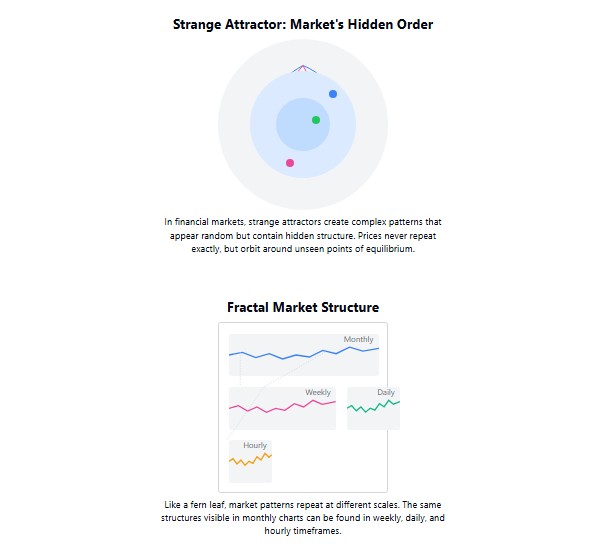
But unlike a simple ball, markets have something that is called "strange attractors." These are not just points, but complex structures that the system strives for, but never repeats itself exactly. Like a stream flowing into a lake, the water always flows towards the lake, but never exactly follows its path.

How to understand the fractal pattern of the market

Benoît B. Mandelbrot, while working for IBM in the 1960s, analyzed long-term fluctuations in cotton prices. He noticed something surprising: price charts looked the same whether he looked at daily, monthly, or yearly data. This discovery led to the development of fractal geometry — the study of shapes that repeat themselves at different scales.

Look at a fern leaf: its general shape is repeated in each small leaflet, and then in even smaller parts. Markets operate in a similar way. The patterns you see on the minute chart are often repeated on the hourly, daily, and even monthly charts.

This self-similarity is not accidental. It reflects the fact that markets are not just random noise, but complex systems with internal structure. And understanding this structure provides us with a key to predicting future movements.

Return to the mean: The universal rhythm of nature

There is a saying in the world of finance: "Trees don't grow to the sky." History shows us that after periods of extreme growth or decline, markets tend to revert to their long-term average.

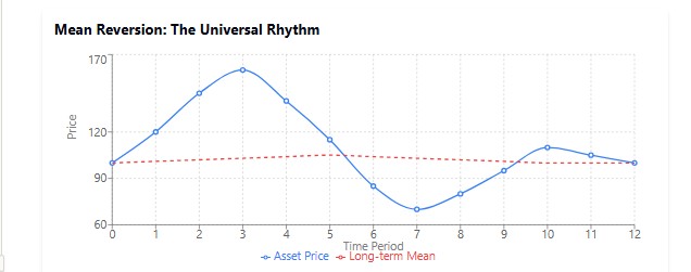
This phenomenon can be observed everywhere in nature. Imagine a pendulum: the further you swing it, the more it tries to return to the center position. Or think about your body temperature: when you have a fever, your body is working to bring your temperature back down to the normal 36.6°C.

This effect is constantly evident in the markets. Stocks that show extraordinary returns in one period often manifest mediocre results in the next one. Companies that grow faster than the market over a long period of time almost inevitably slow down. As a legendary investor, Peter Lynch noted, "Reversion to the mean is a force of gravity that even great companies cannot escape."

But what makes the Sensory Neural Attractor revolutionary is its ability to identify not just a static average, but the dynamic level that the market is currently moving towards. It's like being able to predict exactly where a pendulum will stop if gravity suddenly changes.

Sensitivity to initial conditions: The butterfly effect on Wall Street

"Can the flapping of butterfly's wings in Brazil cause a tornado in Texas?" Lorenz's famous question illustrates a key principle of chaos theory: sensitivity to initial conditions.

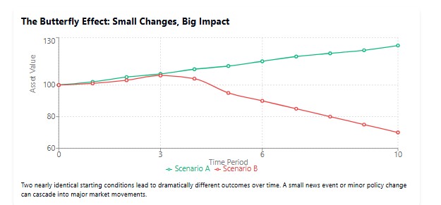
We see these "butterfly effects" all the time in financial markets. A CEO's tweet could send the company's stock crashing. An unexpected decision by the Federal Reserve could trigger a global correction. Even rumors of problems at a small bank can result in panic throughout the banking sector, as we saw during the 2008 crisis.

This sensitivity makes accurate long-term forecasting impossible. As Niels Bohr joked: "Predicting is very difficult, especially the future." However, by understanding the structure of the system and identifying attractors, we can make probabilistic predictions that provide an advantage.

Neural attractor oscillator: Taming market chaos

From theory to practice: Creating an indicator

Have you ever noticed how the price of an asset seems to return to a certain level, as if driven by an invisible force? How does a sharp correction follow a wild rally, or how does a sudden recovery begin after a prolonged decline? It's as if something invisible is pulling the price back, preventing it from moving in one direction forever. It is this invisible force that we intend to catch in our digital net.

While other traders continue to use indicators from the last century, we will embark on a deeper journey – to create an indicator that literally learns to recognize the hidden rhythm of the market. Our compass on this journey will be a neural network, and our map will be the attractor theory.

Neural network architecture: The brain of our indicator

Remember how in movies about hackers the main character creates a superintelligence in a couple of minutes of screen time? In practice, everything is a bit more complicated, but not so much that an ordinary trader-programmer cannot do it.

Our neural network can be thought of as an experienced tracker that analyzes tracks in the snow — historical prices — and tries to predict where the animal (the market) is heading. The structure of this tracker is quite simple: an input layer that collects data, a hidden layer where the pattern recognition "magic" happens, and an output layer that makes the prediction.

This is what the initialization of our brain center looks like:

void InitializeNetwork() {
   // Initializing hidden layer
   ArrayResize(Network.hidden, HiddenNeurons);
   for(int i = 0; i < HiddenNeurons; i++) {
      ArrayResize(Network.hidden[i].weights, InputNeurons);
      // Initializing weights with random values in the range [-0.5, 0.5]
      for(int j = 0; j < InputNeurons; j++) {
         Network.hidden[i].weights[j] = (MathRand() / 32767.0) - 0.5;
      }
      Network.hidden[i].bias = (MathRand() / 32767.0) - 0.5;
   }
   
   // Initializing output neuron
   ArrayResize(Network.output.weights, HiddenNeurons);
   for(int i = 0; i < HiddenNeurons; i++) {
      Network.output.weights[i] = (MathRand() / 32767.0) - 0.5;
   }
   Network.output.bias = (MathRand() / 32767.0) - 0.5;
}

Pay attention to the lines where weights are initialized. It's like adjusting microscope sensitivity before a research. We start with random values, and then the learning process gradually adjusts these "tuning knobs" to produce a more accurate image.

Network training: From novice to master

Imagine a child learning to walk. First he falls, then takes a few steps, falls again, but gradually improves his skills. In the same way, our network learns to "walk" using historical data, constantly adjusting its steps.

The key part of this process is the forward and reverse passes. In the forward pass, the network makes a prediction; while in the reverse pass, it adjusts its weights depending on the error.

double ForwardPass(double &inputs[]) {
   // Calculating outputs of the hidden layer
   for(int i = 0; i < HiddenNeurons; i++) {
      double sum = Network.hidden[i].bias;
      for(int j = 0; j < InputNeurons; j++) {
         sum += inputs[j] * Network.hidden[i].weights[j];
      }
      Network.hidden[i].output = Sigmoid(sum);
   }
   
   // Calculating neural network output
   double sum = Network.output.bias;
   for(int i = 0; i < HiddenNeurons; i++) {
      sum += Network.hidden[i].output * Network.output.weights[i];
   }
   Network.output.output = Sigmoid(sum);
   
   return Network.output.output;
}

If we could look inside this function while it was running, we would see something akin to electrical impulses passing through brain neurons – information passing through a network of connections, being transformed and amplified.

Activation function: firing neurons

In the updated version of the indicator, we replaced the classic sigmoid with hyperbolic tangent (tanh). This function has the range [-1, 1], which makes it particularly effective for modeling chaotic systems where both positive and negative values​are important.

double Tanh(double x) {
   return (MathExp(x) - MathExp(-x)) / (MathExp(x) + MathExp(-x));
}

Hyperbolic tangent has a steeper slope in the center, which allows the network to learn faster and more accurately capture sudden changes in the data. This is critical for chaotic markets where transitions between states can occur rapidly.

Data normalization: Speaking the same language

Before feeding data into a neural network, it must be normalized — brought to a common scale. It's like translating a text into a language that is understandable to the interlocutor. If you speak Russian and your interlocutor only understands English, communication will fail.

double NormalizePrice(double price) {
   double min = ArrayMin(PriceHistory);
   double max = ArrayMax(PriceHistory);
   return (price - min) / (max - min);
}

This function scales all prices to the range between 0 and 1, which is perfect for the input of our sigmoid activation function.

Oscillator calculation: The moment of truth

Finally, we have reached the most interesting part - calculating the oscillator value. How do we calculate it? Essentially, we compare the current price with the predicted attractor and express deviation as a percentage.

// Calculate oscillator value as ratio of current price to attractor
if(AttractorBuffer[i] > 0) {
   OscillatorBuffer[i] = (CurrentPriceBuffer[i] / AttractorBuffer[i] - 1.0) * 100.0;
} else {
   OscillatorBuffer[i] = 0; // Division-by-zero protection
}

This simple formula tells us how far the current price has deviated from its "natural" level. If the oscillator shows +30%, the price is "overheated" and may soon return to the attractor. If -30%, the price is "overcooled" and may rebound upwards.

Customize the indicator to suit our needs

Remember the old saying, "One size fits all"? In trading this rarely works. Each market, each timeframe has its own character, its own "mood". And our indicator must adapt to these features.

input int    InputNeurons = 10;     // Number of input neurons (historical periods)
input int    HiddenNeurons = 20;    // Number of neurons in the hidden layer
input double LearningRate = 0.01;   // Learning rate
input int    TrainBars = 1000;      // Number of bars for training
input int    PredictionPeriod = 5;  // Prediction period (in bars)
input bool   Smoothing = false;     // Apply smoothing to the oscillator
input int    SmoothingPeriod = 3;   // Smoothing period

These parameters are like controls on an expensive audio amplifier. Want a more sensitive indicator? Increase the number of neurons or decrease the prediction period. Too much noise? Turn on smoothing.

Prediction period: Looking into the future

The PredictionPeriod parameter is especially interesting. It determines how far into the future we try to look. If you are a scalper working on minute charts, then a value of 5 means a forecast for 5 minutes forward. If you are a positional trader on daily charts, then it is 5 days.

I recommend experimenting with this setting. Start with small values and gradually increase them, observing how the indicator's behavior changes. As in real science, there are no ready-made formulas here - only experience and experiments.

Lyapunov exponent: Measuring market randomness

The key component of our updated indicator is the Lyapunov exponent, a measure of system's sensitivity to initial conditions. This indicator mathematically describes the famous "butterfly effect" - a phenomenon where small changes in initial conditions result in significant divergencies in the long term.

double CalculateLyapunovExponent(const double &close[], int bars) {
   double epsilon = 0.0001; // Small perturbation
   double lyapunov = 0.0;
   int samples = MathMin(LyapunovPeriod, TrainBars/2);
   
   for(int i = 0; i < samples; i++) {
      int startIdx = MathRand() % (TrainBars - InputNeurons - PredictionPeriod);
      
      // Initial input data
      double inputs1[];
      ArrayResize(inputs1, InputNeurons);
      for(int j = 0; j < InputNeurons; j++) {
         inputs1[j] = NormalizePrice(close[bars - TrainBars + startIdx + j]);
      }
      
      // Slightly perturbed input data
      double inputs2[];
      ArrayResize(inputs2, InputNeurons);
      ArrayCopy(inputs2, inputs1);
      inputs2[MathRand() % InputNeurons] += epsilon;
      
      // Predictions for both data sets
      double pred1 = ForwardPass(inputs1);
      double pred2 = ForwardPass(inputs2);
      
      // Distance between predictions
      double distance = MathAbs(pred2 - pred1);
      
      // Lyapunov exponent
      if(distance > 0) {
         lyapunov += MathLog(distance / epsilon);
      }
   }
   
   // Average and normalize
   lyapunov = lyapunov / samples;
   
   // Limit the value for stability
   lyapunov = MathMax(-1.0, MathMin(1.0, lyapunov));
   
   return lyapunov;
}

Fractal noise: Adding natural structure

One of the most innovative elements of our indicator is the inclusion of fractal noise generated by a Midpoint Displacement algorithm. Fractal geometry, first applied to financial markets by Benoit Mandelbrot, enables us to model their natural self-similar structure.

void GenerateFractalNoise(int size) {
   ArrayResize(FractalNoiseBuffer, size);
   
   // Starting points
   FractalNoiseBuffer[0] = 0;
   FractalNoiseBuffer[size-1] = 0;
   
   // Recursive calculation of midpoints
   MidpointDisplacement(FractalNoiseBuffer, 0, size-1, 1.0, FractalDimension);
   
   // Normalization
   double min = ArrayMin(FractalNoiseBuffer, 0, size);
   double max = ArrayMax(FractalNoiseBuffer, 0, size);
   
   for(int i = 0; i < size; i++) {
      FractalNoiseBuffer[i] = 2.0 * (FractalNoiseBuffer[i] - min) / (max - min) - 1.0;
   }
}

The higher the Fractal Dimension (FractalDimension) parameter is, the more jagged and chaotic the noise becomes, allowing for more accurate modeling of highly volatile markets.

Practical application of the indicator

Now that we understand how our indicator works, let's discuss its practical application. Like any oscillator, the Neural Attractor Oscillator can be used to determine if the market is overbought and oversold.

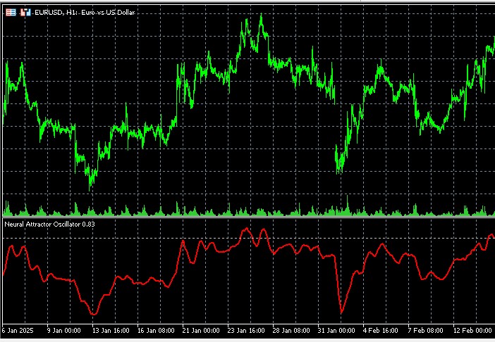
Imagine that you are watching a pendulum. When it deviates too far to the right, you know that soon it will start moving to the left. When it is too far to the left, it will soon go to the right. Our indicator operates the same way, but instead of mechanical forces that return the pendulum to the center, there are equilibrium market forces.

Entry signals subject to chaos

1. Buy signal: When the oscillator drops below the attractor’s lower boundary (which is dynamically adjusted depending on the Lyapunov exponent) and starts to rise, this can be a good point to enter a long position. Whereas, it is important to take into account the current value of the Lyapunov exponent: the lower it is, the more reliable the signal.
2. Sell signal: When the oscillator rises above the attractor’s upper boundary and starts to fall, this may indicate a good point to enter a short position. Again, a low Lyapunov exponent increases the reliability of the signal.
3. Divergencies: A particularly valuable and highly accurate signal of divergence between the indicator peaks and the price.

Remember that during periods of high chaos (high Lyapunov exponent), even strong signals are less reliable, and you should reduce your position size or refrain from entering the market altogether.

Divergencies in the context of chaos theory

The Chaos Attractor Oscillator offers a new perspective on classic divergences. When the price forms a new extreme, but the oscillator does not, this may indicate not just a weakening trend, but a change in the attractor’s structure — the equilibrium point toward which the market is striving.

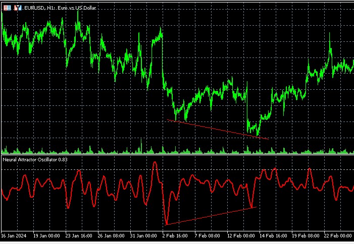
Particularly powerful signals arise when divergence coincides with a change in the Lyapunov exponent. For example, a transition from a positive to a negative value can indicate the formation of a new stable trend after a period of chaos.

Momentum optimization of the network

In our updated indicator, we have applied a Momentum optimization method that significantly enhances the learning process and reduces the likelihood of getting stuck in local minima:

// Updating the output layer weights with momentum
for(int j = 0; j < HiddenNeurons; j++) {
    double delta = LearningRate * Network.output.error * Network.hidden[j].output;
    Network.output.momentum[j] = momentum * Network.output.momentum[j] + (1.0 - momentum) * delta;
    Network.output.weights[j] += Network.output.momentum[j];
}

The Momentum method works like "inertia" in the physical world - if the network has been moving in a certain direction for a long time during optimization, it will continue moving in that direction even when encountering small obstacles (local minima). This is especially useful for chaotic systems, where the error function landscape can be very complex.

Future improvements

While our indicator is already a powerful tool, there are several directions for further development of the chaos attractor concept:

1. Recurrent neural networks: Replacing our feedforward neural network with a recurrent one (LSTM or GRU) can improve the model's ability to capture long-term dependencies in chaotic systems.
2. Multifractal analysis: Implementing multifractal analysis methods to determine the structure of volatility on different time scales.
3. Attractor topology analysis: Applying dynamic topology methods to identification and classification of strange attractors in price dynamics.
4. Quantum algorithms: In the future, quantum computing may be used to model complex chaotic systems, which could lead to revolutionary breakthroughs in predicting market movements.

And of course, later we will definitely consider the issue of creating an expert advisor on this system. This is how a rough draft - the EA sketch - looks like:

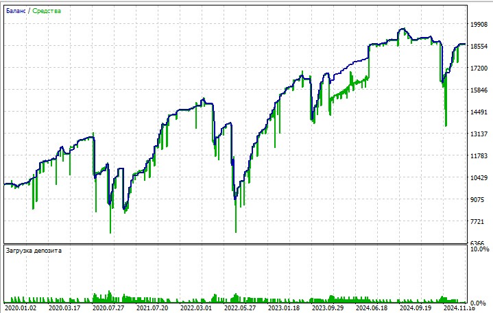
Generally, the system functions quite well, not particularly great, but not terrible either.

Flexible smoothing methods

In the updated version of the indicator, we have added a choice of different smoothing methods, allowing traders to customize the indicator's response based on market conditions:

void ApplySmoothing(int rates_total, int prev_calculated, int period, ENUM_MA_METHOD method) {
   int start = prev_calculated == 0 ? InputNeurons + period : prev_calculated - 1;
   
   double temp[];
   ArrayResize(temp, rates_total);
   ArrayCopy(temp, OscillatorBuffer);
   
   for(int i = start; i < rates_total; i++) {
      switch(method) {
         case MODE_SMA: // Simple moving average
            {
               double sum = 0;
               for(int j = 0; j < period; j++) {
                  sum += temp[i - j];
               }
               OscillatorBuffer[i] = sum / period;
            }
            break;
            
         case MODE_EMA: // Exponential moving average
            {
               double alpha = 2.0 / (period + 1.0);
               OscillatorBuffer[i] = temp[i] * alpha + OscillatorBuffer[i-1] * (1.0 - alpha);
            }
            break;
            
         // ... other methods ...
      }
   }
}

For chaotic markets with a high Lyapunov exponent, it is better to use EMA, which reacts faster to changes. For more predictable markets with a low Lyapunov exponent, SMA can provide more reliable signals with fewer false triggers.

Conclusion

We have created not just another technical indicator, but a complete system for analyzing market chaos. The Chaos Attractor Oscillator combines the latest advances in chaos theory, fractal geometry, and neural networks, providing traders with a tool for navigating complex and unpredictable market conditions.

A particular value of this indicator lies in its ability not only to generate trading signals, but also to evaluate the reliability of these signals through the Lyapunov exponent. This enables the trader to adapt their strategy to the current market conditions – to be aggressive when the system is predictable and cautious when it is chaotic.

In the era of algorithmic trading and artificial intelligence, those who can best model the complex nature of the market gain an advantage. Chaos Attractor Oscillator is a step in that direction, allowing us to see order where others see only randomness.

Remember that even the most advanced indicator is not a magic formula for success. Trading always requires discipline, risk management and understanding of the market context. But by arming yourself with a tool that allows you to peer into the very nature of market chaos, you gain a significant advantage on the path to consistent profits.

Good luck in trading and may the chaos attractors be with you!