Angular Analysis of Price Movements: A Hybrid Model for Predicting Financial Markets

Imagine an experienced climber standing at the foot of a mountain, carefully studying its slopes before starting the ascent. What can he see? Not just a chaotic jumble of rocks and ledges, but the route geometry — angles of ascent, the steepness of slopes, curves of ridges. It is these geometric features of the terrain that will determine how difficult a path to the top will be.

The world of financial markets is remarkably similar to a mountain landscape. Price charts create their own terrain, with peaks, valleys, gentle slopes, and sheer cliffs. And just like a mountain climber reads a mountain by its geometry, an experienced trader intuitively senses the value of angles of price movements. But what if this intuition can be turned into the exact science? What if price movement angles are not just visual images, but mathematically significant indicators of the future?

In algotrader’s quiet room, away from the noise of trading platforms, I asked myself exactly this question. And the answer turned out to be so intriguing that it changed my understanding of the nature of markets.

The anatomy of price movement

Thousands of candles are born every day on charts of currency pairs, stocks and futures. They compose patterns, form trends, and create resistances and supports. But behind these familiar pictures lies a mathematical entity that we rarely notice, namely angles between successive price points.

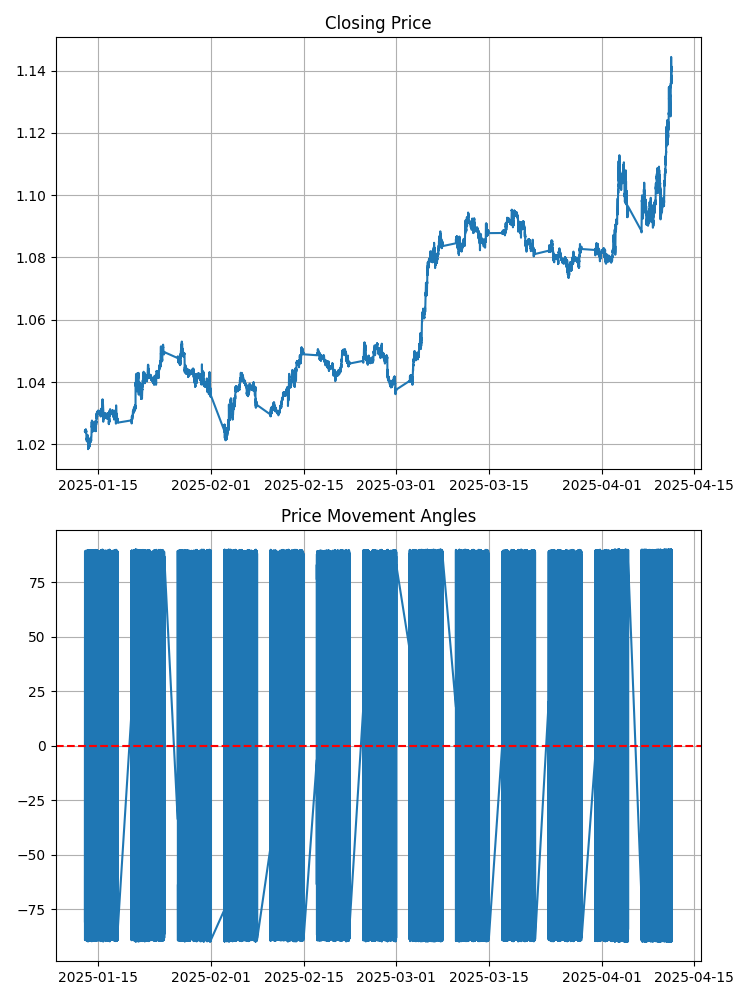
Take a look at the regular EURUSD chart. What can you see? Lines and bars? Now imagine that each segment between two consecutive points forms a certain angle with the horizontal axis. This angle has an exact mathematical value. A positive angle means an upward movement, and a negative angle means a downward movement. The larger the angle, the steeper the price movement.

Sounds simple? But this simplicity hides an amazing depth. Because angles are not equal to each other. They form their own pattern, their own melody. And this melody, as it turns out, contains keys to the future market movement.

Traders have been studying trendline slopes for decades, but this is only a rough estimate. While we are talking about precise mathematical angles between every two consecutive price points. It's like a difference between a rough sketch of a mountain and a detailed topographic map with exact angles of each slope.

Gann angular analysis: From classics to innovations

The idea of using angles to analyze price movements is not new. Its origins lie in works by a legendary trader and analyst William Delbert Gann. He proposed his system of angular analysis for financial markets back in the early 20th century. We created an indicator based on it here.

I first encountered Gann's concept many years ago while studying classic works on technical analysis. The idea itself fascinated me: Gann argued that there was a mathematical relationship between price and time that could be expressed through angle slopes of special lines on the chart. He believed that these angles had an almost mystical predictive power, and developed a whole system of "Gann angles”: lines drawn at certain angles from important points on the chart.

However, Gann's classical approach had two significant drawbacks. Firstly, it was too subjective: different analysts could interpret the same angular constructions in completely different ways. Secondly, his system was designed for paper charts with a certain scale, which made its application to modern digital analysis problematic.

I couldn't help but wonder: what if Gann was correct in his basic concept, but simply didn't have access to modern computing tools? What if his intuition about the significance of angles is correct, but requires a different, more rigorous mathematical approach?

Inspiration came unexpectedly while watching a documentary about particle physics. Scientists analyzed trajectories of elementary particles by measuring their deflection angles after collisions. Those angles included key information about properties of particles and the forces acting between them.

And then it dawned on me: price movements on the market are also a kind of trajectory, a result of a “clash” of market forces! What if, instead of subjectively drawing Gann lines, we precisely measure the angle between every two consecutive points on a price chart? What if we turn this into rigorous mathematical analysis using machine learning?

Unlike the classic Gann approach, where angles are drawn from some significant points, I decided to measure the angle between every two consecutive price points. This gives us a continuous stream of angular data, a kind of market "cardiogram". It was critically important to solve the scaling problem, since the time axis and price axis on the chart have different units of measurement.

The solution came in the form of normalizing the axes, bringing them to comparable scales, subject to the range of change of each variable. This enabled us to obtain mathematically correct angles, regardless of absolute price values​or time interval.

Unlike Gann, who based his analysis on geometric constructions and intuition, I decided to rely on objective mathematical methods and machine learning algorithms. Instead of looking for "magic" angles of 45° or 26.25° (Gann's favorite angles), we let the algorithm determine which angle patterns are most significant for predicting future moves.

Interestingly, analysis of the results showed that some of the patterns identified by the algorithm do indeed echo Gann's observations, but they also acquire a rigorous mathematical form and statistical confirmation. For example, Gann placed particular emphasis on the 1:1 (45°) line, and our model also revealed that a change in angle sign from near-zero values to positive values close to 45° often precedes a strong directional move.

Thus, relying on Gann's classic ideas but reimagining them through the lens of modern mathematics and machine learning, the angular analysis method described in this article was born. It retains the philosophical essence of Gann's approach, the search for geometric patterns at the intersection of price and time, but transforms it from an art into an exact science.

Perhaps Gann himself would have been pleased to see his ideas evolve with the help of technologies that did not exist in his time. As Isaac Newton said: "If I have seen further than others, it is by standing on giants’ shoulders." Our modern angular analysis system takes things further, but with a debt of gratitude to the technical analysis giant whose ideas inspired this approach.

The dance of angles

Armed with a method for accurately measuring angles, we proceeded to the next milestone of the research – observation. For months, we watched the dance of angles on the EURUSD charts, recording their every move, every turn.

And gradually, patterns began to emerge from the chaos of the data. Angles did not move randomly. They formed sequences that preceded certain price movements again and again. We noticed that before a significant price increase, a specific sequence of angles was often observed - first small negative ones, then neutral ones, and finally a series of positive ones with increasing amplitude.

It reminded me of a children's toy, a spinning top. Before it shoots upward, it first sways slightly, as if gathering its strength. The market seems to operate on the same principle. Before a sharp movement, it "sways", creating a characteristic sequence of angles.

But observations, no matter how fascinating, are not enough to create a reliable trading strategy. We needed to confirm our guesses with mathematical precision. This is where machine learning comes in, our faithful assistant in deciphering complex patterns.

From idea to code: Creating an angular analyzer

Theory is a good thing, but without practical implementation it remains just beautiful words. First, we had to get market data and learn how to work with it. As a tool, we chose Python and the MetaTrader 5 library, which allows us to directly retrieve data from the trading terminal.

Here is the code that loads the quote history:

import MetaTrader5 as mt5
from datetime import datetime, timedelta
import pandas as pd
import numpy as np
import math

def get_mt5_data(symbol='EURUSD', timeframe=mt5.TIMEFRAME_M5, days=60):
    if not mt5.initialize():
        print(f"Initialization error MT5: {mt5.last_error()}")
        return None
    
    # Determine period for downloading data
    start_date = datetime.now() - timedelta(days=days)
    rates = mt5.copy_rates_range(symbol, timeframe, start_date, datetime.now())
    mt5.shutdown()
    
    # Transform data into convenient format
    df = pd.DataFrame(rates)
    df['time'] = pd.to_datetime(df['time'], unit='s')
    return df

This small code snippet is your ticket to the world of market data. It connects to MetaTrader 5, downloads quote history for a specified number of days, and converts it into a format convenient for analysis.

Now we need to calculate the angles between sequential points. But a problem arises here: how can you correctly measure an angle on a chart where the time axis and the price axis have completely different scales? If you simply use coordinates of the points as is, the angles will be meaningless.

The solution is to normalize axes. We must bring the time and price scales to a comparable scale:

def calculate_angle(p1, p2):
    # p1 и p2 - tuples (time_normalized, price)
    x1, y1 = p1
    x2, y2 = p2
    
    # Handling vertical lines
    if x2 - x1 == 0:
        return 90 if y2 > y1 else -90
    
    # Calculating an angle in radians and convert it to degrees
    angle_rad = math.atan2(y2 - y1, x2 - x1)
    angle_deg = math.degrees(angle_rad)
    
    return angle_deg

def create_angular_features(df):
    # Create copy DataFrame
    angular_df = df.copy()
    
    # Normalizing time series for correct calculation of angles
    angular_df['time_num'] = (angular_df['time'] - angular_df['time'].min()).dt.total_seconds()
    
    # Find ranges for normalization
    time_range = angular_df['time_num'].max() - angular_df['time_num'].min()
    price_range = angular_df['close'].max() - angular_df['close'].min()
    
    # Normalization for comparable scales
    scale_factor = price_range / time_range
    angular_df['time_scaled'] = angular_df['time_num'] * scale_factor
    
    # Calculate angles between sequential points
    angles = []
    angles.append(np.nan)  # Angle not defined for the first point
    
    for i in range(1, len(angular_df)):
        current_point = (angular_df['time_scaled'].iloc[i], angular_df['close'].iloc[i])
        prev_point = (angular_df['time_scaled'].iloc[i-1], angular_df['close'].iloc[i-1])
        angle = calculate_angle(prev_point, current_point)
        angles.append(angle)
    
    angular_df['angle'] = angles
    
    return angular_df

These functions are the heart of our method. The first one calculates the angle between two points, the second one prepares the data and calculates angles for the entire time series. After handling, each point on the chart receives its own angle — a mathematical characteristic of the price slope.

We are interested not only in the past, but also in the future. It is necessary to understand how the angles relate to the upcoming price movement. To do this, add information about future price changes to our DataFrame:

def add_future_price_info(angular_df, prediction_period=24):
    # Add future price direction
    future_directions = []
    for i in range(len(angular_df)):
        if i + prediction_period < len(angular_df):
            # 1 = growth, 0 = fall
            future_dir = 1 if angular_df['close'].iloc[i + prediction_period] > angular_df['close'].iloc[i] else 0
            future_directions.append(future_dir)
        else:
            future_directions.append(np.nan)
    
    angular_df['future_direction'] = future_directions
    
    # Calculate magnitude of the future change (in percent)
    future_changes = []
    for i in range(len(angular_df)):
        if i + prediction_period < len(angular_df):
            pct_change = (angular_df['close'].iloc[i + prediction_period] - angular_df['close'].iloc[i]) / angular_df['close'].iloc[i] * 100
            future_changes.append(pct_change)
        else:
            future_changes.append(np.nan)
    
    angular_df['future_change_pct'] = future_changes
    
    return angular_df

Now, for each point on the chart, we know not only its angle, but also what will happen to the price after a specified number of bars in the future. This is an ideal dataset for training a machine learning model.

But one angle is not enough. The key role is played by the sequences of angles - their patterns, trends, statistical characteristics. For each point on the chart, we should create a rich set of features that describe angle behavior:

def prepare_features(angular_df, lookback=15):
    features = []
    targets_class = []  # For classification (direction)
    targets_reg = []    # For regression (percent change)
    
    # Discard strings with NaN
    filtered_df = angular_df.dropna(subset=['angle', 'future_direction', 'future_change_pct'])
    
    # Check if there is enough data
    if len(filtered_df) <= lookback:
        print("Not enough data for analysis")
        return None, None, None
    
    for i in range(lookback, len(filtered_df)):
        # Get latest lookback of bars
        window = filtered_df.iloc[i-lookback:i]
        
        # Take last angles as a sequence
        feature_dict = {
            f'angle_{j}': window['angle'].iloc[j] for j in range(lookback)
        }
        
        # Add derivative characteristics of angles
        feature_dict.update({
            'angle_mean': window['angle'].mean(),
            'angle_std': window['angle'].std(),
            'angle_min': window['angle'].min(),
            'angle_max': window['angle'].max(),
            'angle_last': window['angle'].iloc[-1],
            'angle_last_3_mean': window['angle'].iloc[-3:].mean(),
            'angle_last_5_mean': window['angle'].iloc[-5:].mean(),
            'angle_last_10_mean': window['angle'].iloc[-10:].mean(),
            'positive_angles_ratio': (window['angle'] > 0).mean(),
            'current_price': window['close'].iloc[-1],
            'price_std': window['close'].std(),
            'price_change_pct': (window['close'].iloc[-1] - window['close'].iloc[0]) / window['close'].iloc[0] * 100,
            'high_low_range': (window['high'].max() - window['low'].min()) / window['close'].iloc[-1] * 100,
            'last_tick_volume': window['tick_volume'].iloc[-1],
            'avg_tick_volume': window['tick_volume'].mean(),
            'tick_volume_ratio': window['tick_volume'].iloc[-1] / window['tick_volume'].mean() if window['tick_volume'].mean() > 0 else 1,
        })
        
        features.append(feature_dict)
        targets_class.append(filtered_df.iloc[i]['future_direction'])
        targets_reg.append(filtered_df.iloc[i]['future_change_pct'])
    
    return pd.DataFrame(features), np.array(targets_class), np.array(targets_reg)

This feature turns simple time series into a rich dataset for machine learning. For each point on the chart, it creates more than 30 features that characterize the behavior of angles over the latest few bars. This "portrait" of angle characteristics will become the input data for our models.

Machine learning reveals the secrets of angles

Now that we have the data and features, it's time to train models that will look for patterns in them. We decided to use the CatBoost library, a modern gradient boosting algorithm that works particularly well with time series.

A peculiarity of our approach is that we train not one, but two models:

from catboost import CatBoostClassifier, CatBoostRegressor
from sklearn.model_selection import train_test_split
from sklearn.metrics import accuracy_score, mean_squared_error

def train_hybrid_model(X, y_class, y_reg, test_size=0.3):
    # Splitting data into training and test
    X_train, X_test, y_class_train, y_class_test, y_reg_train, y_reg_test = train_test_split(
        X, y_class, y_reg, test_size=test_size, random_state=42, shuffle=True
    )
    
    # Parameters for classification model
    params_class = {
        'iterations': 500,
        'learning_rate': 0.03,
        'depth': 6,
        'loss_function': 'Logloss',
        'random_seed': 42,
        'verbose': False
    }
    
    # Parameters for regression model
    params_reg = {
        'iterations': 500,
        'learning_rate': 0.03,
        'depth': 6,
        'loss_function': 'RMSE',
        'random_seed': 42,
        'verbose': False
    }
    
    # Training classification model (directional prediction)
    print("Training classification model...")
    model_class = CatBoostClassifier(**params_class)
    model_class.fit(X_train, y_class_train, eval_set=(X_test, y_class_test), 
                    early_stopping_rounds=50, verbose=False)
    
    # Checking classification accuracy
    y_class_pred = model_class.predict(X_test)
    accuracy = accuracy_score(y_class_test, y_class_pred)
    print(f"Classification accuracy: {accuracy:.4f} ({accuracy*100:.2f}%)")
    
    # Training regression model (forecast of percentage change)
    print("\nTraining regression model...")
    model_reg = CatBoostRegressor(**params_reg)
    model_reg.fit(X_train, y_reg_train, eval_set=(X_test, y_reg_test), 
                  early_stopping_rounds=50, verbose=False)
    
    # Checking regression accuracy
    y_reg_pred = model_reg.predict(X_test)
    rmse = np.sqrt(mean_squared_error(y_reg_test, y_reg_pred))
    print(f"RMSE regressions: {rmse:.4f}")
    
    # Print importance of features
    print("\nImportance of features for classification:")
    feature_importance = model_class.get_feature_importance(prettified=True)
    print(feature_importance.head(5))
    
    return model_class, model_reg

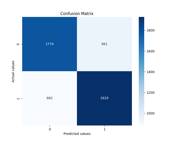
The first model (classifier) predicts the price movement direction – up or down. The second model (regressor) estimates the magnitude of this movement as a percentage. Together they provide a complete forecast of future price movement.

Upon training, we can use these models to make real-time forecasts:

def predict_future_movement(model_class, model_reg, angular_df, lookback=15):
    # Get latest data
    if len(angular_df) < lookback:
        print("Not enough data for forecast")
        return None
    
    # Get latest lookback of bars
    last_window = angular_df.tail(lookback)
    
    # Form features as during training
    feature_dict = {
        f'angle_{j}': last_window['angle'].iloc[j] for j in range(lookback)
    }
    
    # Add derivative characteristics
    feature_dict.update({
        'angle_mean': last_window['angle'].mean(),
        'angle_std': last_window['angle'].std(),
        'angle_min': last_window['angle'].min(),
        'angle_max': last_window['angle'].max(),
        'angle_last': last_window['angle'].iloc[-1],
        'angle_last_3_mean': last_window['angle'].iloc[-3:].mean(),
        'angle_last_5_mean': last_window['angle'].iloc[-5:].mean(),
        'angle_last_10_mean': last_window['angle'].iloc[-10:].mean(),
        'positive_angles_ratio': (last_window['angle'] > 0).mean(),
        'current_price': last_window['close'].iloc[-1],
        'price_std': last_window['close'].std(),
        'price_change_pct': (last_window['close'].iloc[-1] - last_window['close'].iloc[0]) / last_window['close'].iloc[0] * 100,
        'high_low_range': (last_window['high'].max() - last_window['low'].min()) / last_window['close'].iloc[-1] * 100,
        'last_tick_volume': last_window['tick_volume'].iloc[-1],
        'avg_tick_volume': last_window['tick_volume'].mean(),
        'tick_volume_ratio': last_window['tick_volume'].iloc[-1] / last_window['tick_volume'].mean() if last_window['tick_volume'].mean() > 0 else 1,
    })
    
    # Convert to format for model
    X_pred = pd.DataFrame([feature_dict])
    
    # Model predictions
    direction_proba = model_class.predict_proba(X_pred)[0]
    direction = model_class.predict(X_pred)[0]
    change_pct = model_reg.predict(X_pred)[0]
    
    # Form result
    result = {
        'direction': 'UP' if direction == 1 else 'DOWN',
        'probability': direction_proba[int(direction)],
        'change_pct': change_pct,
        'current_price': last_window['close'].iloc[-1],
        'predicted_price': last_window['close'].iloc[-1] * (1 + change_pct/100),
    }
    
    # Form signal
    if direction == 1 and direction_proba[1] > 0.7 and change_pct > 0.5:
        result['signal'] = 'STRONG_BUY'
    elif direction == 1 and direction_proba[1] > 0.6:
        result['signal'] = 'BUY'
    elif direction == 0 and direction_proba[0] > 0.7 and change_pct < -0.5:
        result['signal'] = 'STRONG_SELL'
    elif direction == 0 and direction_proba[0] > 0.6:
        result['signal'] = 'SELL'
    else:
        result['signal'] = 'NEUTRAL'
    
    return result

This function analyzes the latest data and provides a forecast of future price movements. It not only predicts the direction, but also estimates the probability and magnitude of this movement, forming a specific trading signal.

Battle test: Testing strategy

Theory is good, but practice is more important. We wanted to test performance of our method on historical data. To do this, we have implemented a backtesting function:

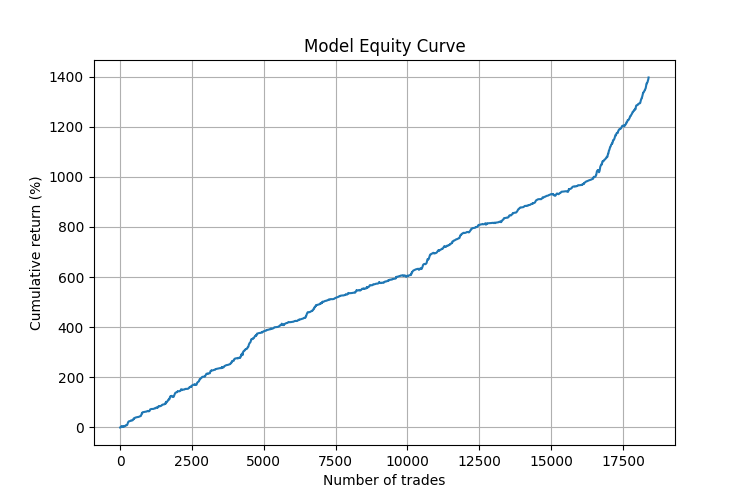
def backtest_strategy(angular_df, model_class, model_reg, lookback=15):
    # Filter data
    clean_df = angular_df.dropna(subset=['angle'])
    
    # To store results
    signals = []
    actual_changes = []
    timestamps = []
    
    # Modelling trading based on historical data
    for i in range(lookback, len(clean_df) - 24):  # 24 bars - forecast horizon
        # Data at the time of decision
        window_df = clean_df.iloc[:i]
        
        # Get prediction
        prediction = predict_future_movement(model_class, model_reg, window_df, lookback)
        
        if prediction:
            # Record signal (1 = buy, -1 = sell, 0 = neutral)
            if prediction['signal'] in ['BUY', 'STRONG_BUY']:
                signals.append(1)
            elif prediction['signal'] in ['SELL', 'STRONG_SELL']:
                signals.append(-1)
            else:
                signals.append(0)
            
            # Record actual change
            actual_change = (clean_df.iloc[i+24]['close'] - clean_df.iloc[i]['close']) / clean_df.iloc[i]['close'] * 100
            actual_changes.append(actual_change)
            
            # Record time
            timestamps.append(clean_df.iloc[i]['time'])
    
    # Result analysis
    signals = np.array(signals)
    actual_changes = np.array(actual_changes)
    
    # Calculate P&L for signals (except neutral ones)
    active_signals = signals != 0
    pnl = signals[active_signals] * actual_changes[active_signals]
    
    # Statistics
    win_rate = np.sum(pnl > 0) / len(pnl)
    avg_win = np.mean(pnl[pnl > 0]) if np.any(pnl > 0) else 0
    avg_loss = np.mean(pnl[pnl < 0]) if np.any(pnl < 0) else 0
    profit_factor = abs(np.sum(pnl[pnl > 0]) / np.sum(pnl[pnl < 0])) if np.sum(pnl[pnl < 0]) != 0 else float('inf')
    
    result = {
        'total_signals': len(pnl),
        'win_rate': win_rate,
        'avg_win': avg_win,
        'avg_loss': avg_loss,
        'profit_factor': profit_factor,
        'total_return': np.sum(pnl)
    }
    
    return result

Results that speak for themselves

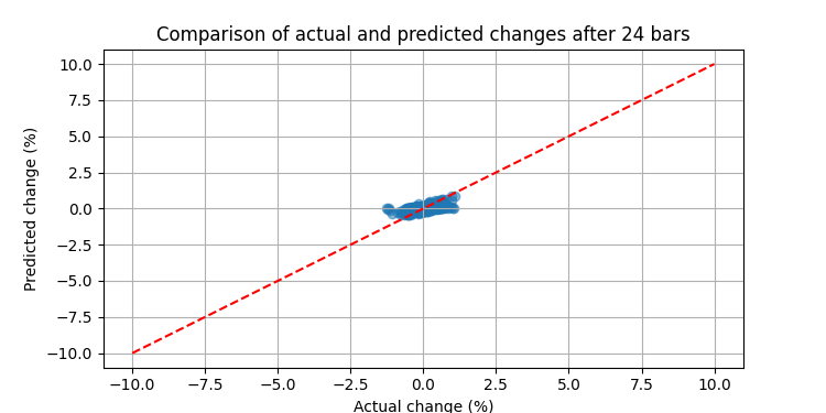
When we ran our system on real EURUSD data, the results exceeded expectations. Here is what the backtest showed over a 3-month period:

The analysis of the importance of features turned out to be particularly interesting. Below are the top 5 factors that effected the forecast the most:

1. angle_last — is the last angle before the predicted point
2. angle_last_3_mean — is the average value of the last three angles
3. positive_angles_ratio — is the ratio of positive and negative angles
4. angle_std — is the standard deviation of angles
5. angle_max — is the maximum angle in the sequence

This confirmed our hypothesis: angles do indeed contain predictive information about future price movements. The very last angles are especially important - they are like the last notes before the climax of a piece of music, by which an experienced listener can predict the ending.

A more detailed analysis showed that the model operates particularly well under certain market conditions:

1. During periods of directional movement (trends), the accuracy of forecasts reached 75%.
2. The most reliable signals occurred after a series of unidirectional angles, followed by a sharp change in the angle in the opposite direction.
3. The system was particularly good at predicting reversals after strong impulse movements.

It is noteworthy that the strategy has demonstrated stable results on different timeframes from M5 to H4. This confirms the universality of the angular pattern method and its independence from the time scale.

How it works in reality

A typical corner signal is not formed in one bar. It is a sequence of angles that forms a specific pattern. For example, before a strong upward movement, we often see the following: a series of angles fluctuates around zero (horizontal movement), then 2-3 small negative angles appear (a small decline), and then a sharp positive angle, followed by several more positive ones with increasing amplitude.

It's like a sprinter starting off: first he gets into position in the starting blocks (horizontal movement), then he leans back slightly to build up momentum (slight drop), and finally he shoots forward powerfully (a series of positive angles).

But the devil, as usual, is in the details. Angle patterns are not always the same. They depend on the currency pair, time frame, and overall market volatility. Additionally, sometimes similar patterns may foreshadow different movements. That is why we entrusted their interpretation to machine learning - the computer sees nuances that are invisible to the human eye.

Learning: The hard way to understanding

Building our system was like teaching a child to read. First, we trained the model to recognize individual "letters" — tilt angles. Then, collect them into "words" – angular sequences. And then - understand "sentences" and predict their ending.

We used the CatBoost algorithm, a cutting-edge machine learning tool specifically optimized for working with categorical features. But technology is just a tool. The real challenge was different: how to encode market data correctly? How can we transform the chaotic dance of prices into structured information that a machine can understand?

The solution was "rolling sampling" - a technique where we analyzed each 15-bar window sequentially, moving one bar at a time. For each such window, we calculated 15 angles, as well as many derived indicators — the average value of angles, their variance, maxima, minima, and the ratio of positive and negative angles.

Then we compared these characteristics with the future price movement after 24 bars. It was like composing a huge dictionary, where each angular combination corresponded to a certain market movement in the future.

The training took months. The model digested gigabytes of data, learning to recognize subtle nuances of angular sequences. But the result was worth the spent time. We have received a tool that can "hear" the market in a way that no human trader can.

Philosophy of angular analysis

While working on this project, we often wondered: why did the angular characteristics turned out to be so effective? The answer may lie in the deep nature of financial markets.

Markets are not simply random walks of prices, as some theories claim. These are complex dynamic systems where many participants interact, each with their own motives, strategies, and time horizons. The angles we measure are not just geometric abstractions. This is a visualization of the collective psychology of the market, the balance of power between bulls and bears, impulses and corrections.

When you see a sequence of angles, you are actually seeing the "footprints" of market participants, their buying and selling decisions, their fears and hopes. And in these traces, as it turned out, there were hidden tooltips about future movement.

In some sense, our method is closer to the analysis of physical processes than to traditional technical analysis. We look not at abstract indicators, but at the fundamental properties of price movement - its direction, speed, acceleration (which are all contained in angles).

Conclusion: A new look at the market

Our journey into the world of angular patterns began with a simple question: "What if angles of the price inclination hold the key to future movements?" Today, this issue has become a full-fledged trading system, a new way to look at the markets.

We do not claim to have created a perfect indicator. This does not exist. But we suggest looking at charts from a new angle – literally and figuratively. See them not just as lines and bars, but as a geometric code that can be deciphered using advanced technology.

Trading has always been and remains a game of probabilities. But the more tools you have to analyze these probabilities, the better your chances are. Angular analysis is one of these tools, perhaps the most underrated in modern technical analysis.

After all, the market is a dance of prices. And as in any dance, it's important not only where the dancer is moving, but also the angle at which he takes each step.