Integrating Computer Vision into Trading in MQL5 (Part 1): Creating Basic Functions

Introduction

In the quiet glow of monitors, where candlestick charts trace the winding paths of financial flows, a new era of trading is being born. Have you ever wondered what a neural network feels when it looks at the EURUSD market? How does it perceive every spike in volatility, every trend reversal, every elusive pattern formation?

Imagine a computer that does not just mindlessly apply pre-programmed rules, but truely sees the market — capturing subtle nuances of price movements that are invisible to the human eye. Artificial intelligence that looks at the EURUSD chart the way an experienced captain looks at the ocean horizon, sensing an approaching storm long before the first signs of bad weather occur.

Today, I invite you on a journey to the cutting edge of financial technology, where computer vision meets market analytics. We will create a system that does not simply analyze the market — it understands it visually, recognizing complex price patterns as naturally as you recognize a friend's face in a crowd.

In a world where milliseconds decide the fate of millions, our model based on convolutional neural networks opens the door to a new dimension of technical analysis. It does not use standard indicators, it learns to find and interpret signals directly from raw OHLC data. And the most amazing thing is that we can look inside its "consciousness" and see which particular chart snippets attract its attention before making a decision.

History and applications of computer vision models

Computer vision was born in the 1960s at Massachusetts Institute of Technology (MIT), when researchers first tried to teach machines to interpret visual information. Initially, development was slow: the first systems could only recognize simple shapes and contours.

The real breakthrough came in 2012 with the advent of deep convolutional neural networks (CNNs), which revolutionized the industry. The AlexNet architecture demonstrated unprecedented image recognition accuracy at the ImageNet competition, thereby ushering in the era of deep learning.

Today, computer vision is transforming many industries. In medicine, algorithms analyze X-rays and MRIs with an accuracy comparable to that of experienced radiologists. In the automotive industry, driver assistance systems and autopilots use CV to recognize road objects. Smartphones use the technology to enhance photos and enable face unlock. Security systems use facial recognition for access control.

The application of computer vision in financial analysis is a new and promising area. CV algorithms are capable of recognizing complex chart patterns and formations that traditional technical indicators cannot, opening up new horizons for algorithmic trading.

Technological foundation: Connecting to market data

Our journey begins with establishing a living connection with the market. Like nerve endings reaching out to the pulse of financial flows, our code connects to the MetaTrader 5 terminal, which is a classic trader's tool that has now become a portal for artificial intelligence:

import MetaTrader5 as mt5
import matplotlib
matplotlib.use('Agg')  # Using Agg backend for running without GUI
import matplotlib.pyplot as plt
from tensorflow.keras.models import Sequential, Model
from tensorflow.keras.layers import Dense, Conv1D, MaxPooling1D, Flatten, Dropout, BatchNormalization, Input

# Connecting to MetaTrader5 terminal
def connect_to_mt5():
    if not mt5.initialize():
        print("Error initializing MetaTrader5")
        mt5.shutdown()
        return False
    return True

The first lines of code are a handshake between the world of algorithms and the world of finance. It might seem like a simple function call, but behind it lies the creation of a channel through which gigabytes of market data, quotations formed at the intersection of millions of traders’ decisions from all over the world will flow.

Our system will use the Agg backend for visualization without a GUI. It is a small but important detail that enables it to run in the background on remote servers without interrupting its vigilant monitoring of the market, even for a second.

Diving into history: Data collection and preparation

Any artificial intelligence starts with data. For our system, these are thousands of EURUSD hourly candles, which are silent witnesses to past price battles, harboring patterns we seek to uncover:

def get_historical_data(symbol="EURUSD", timeframe=mt5.TIMEFRAME_H1, num_bars=1000):
    now = datetime.now()
    from_date = now - timedelta(days=num_bars/24)  # Approximate for hourly bars
    
    rates = mt5.copy_rates_range(symbol, timeframe, from_date, now)
    if rates is None or len(rates) == 0:
        print("Error loading historical quotes")
        return None
    
    # Convert to pandas DataFrame
    rates_frame = pd.DataFrame(rates)
    rates_frame['time'] = pd.to_datetime(rates_frame['time'], unit='s')
    rates_frame.set_index('time', inplace=True)
    
    return rates_frame

This function is where the first magic happens: raw bytes are turned into an ordered stream of data. Every candle, every price fluctuation becomes a point in a multidimensional space that our neural network will explore. We load 2,000 bars of history. It is enough for the model to capture a variety of market conditions, from calm trends to chaotic periods of high volatility.

But computer vision requires not just numbers, but images. The next step is transforming time series into "images" that our convolutional network can analyze:

def create_images(data, window_size=48, prediction_window=24):
    images = []
    targets = []
    
    # Using OHLC data to create images
    for i in range(len(data) - window_size - prediction_window):
        window_data = data.iloc[i:i+window_size]
        target_data = data.iloc[i+window_size:i+window_size+prediction_window]
        
        # Normalize data in the window
        scaler = MinMaxScaler(feature_range=(0, 1))
        window_scaled = scaler.fit_transform(window_data[['open', 'high', 'low', 'close']])
        
        # Predict price direction (up/down) for the forecast period
        price_direction = 1 if target_data['close'].iloc[-1] > window_data['close'].iloc[-1] else 0
        
        images.append(window_scaled)
        targets.append(price_direction)
    
    return np.array(images), np.array(targets)

This is data alchemy in its purest form. We take a window of 48 sequential price bars, normalize their values to a range between 0 and 1, and convert them into a multi-channel image, where each channel corresponds to one of the OHLC components. For each such "frame" of market history, we determine a target value - the direction of price movement 24 bars into the future.

A sliding window sequentially moves through the entire dataset, creating thousands of examples for training. It's like an experienced trader scrolling through historical charts, absorbing market patterns and learning to recognize situations that precede significant moves.

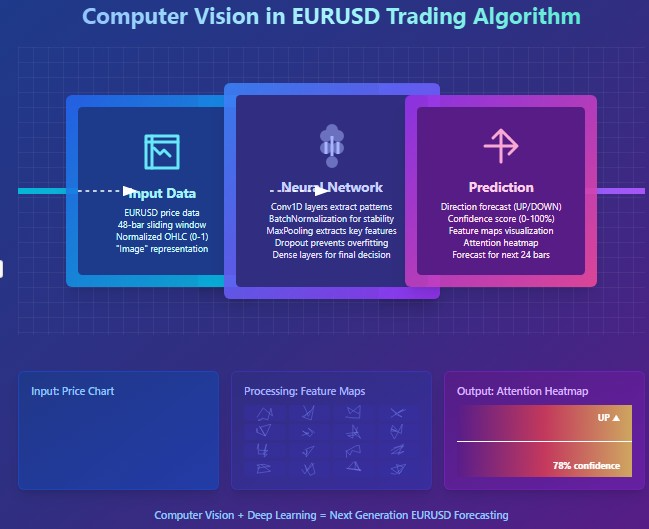
Designing a neural "eye": Model architecture

Now let us proceed to creating the proper neural network. It is an artificial eye that will peer into the chaos of market data in search of hidden order. Our architecture is inspired by recent advances in computer vision, but adapted to the specifics of financial time series:

def train_cv_model(images, targets):
    # Split data into training and validation sets
    X_train, X_val, y_train, y_val = train_test_split(images, targets, test_size=0.2, shuffle=True, random_state=42)
    
    # Create model with improved architecture
    inputs = Input(shape=X_train.shape[1:])
    
    # First convolutional block
    x = Conv1D(filters=64, kernel_size=3, padding='same', activation='relu')(inputs)
    x = BatchNormalization()(x)
    x = Conv1D(filters=64, kernel_size=3, padding='same', activation='relu')(x)
    x = BatchNormalization()(x)
    x = MaxPooling1D(pool_size=2)(x)
    x = Dropout(0.2)(x)
    
    # Second convolutional block
    x = Conv1D(filters=128, kernel_size=3, padding='same', activation='relu')(x)
    x = BatchNormalization()(x)
    x = Conv1D(filters=128, kernel_size=3, padding='same', activation='relu')(x)
    x = BatchNormalization()(x)
    x = MaxPooling1D(pool_size=2)(x)
    feature_maps = x  # Store feature maps for visualization
    x = Dropout(0.2)(x)
    
    # Output block
    x = Flatten()(x)
    x = Dense(128, activation='relu')(x)
    x = BatchNormalization()(x)
    x = Dropout(0.3)(x)
    x = Dense(64, activation='relu')(x)
    x = BatchNormalization()(x)
    x = Dropout(0.3)(x)
    outputs = Dense(1, activation='sigmoid')(x)
    
    # Create the full model
    model = Model(inputs=inputs, outputs=outputs)
    
    # Create a feature extraction model for visualization
    feature_model = Model(inputs=model.input, outputs=feature_maps)

We use the Keras functional API instead of a sequential model. This gives us flexibility to create an additional model that extracts intermediate representations for visualization. This is a key element of our approach: we are not only creating a predictive system, but also a tool for peering into the "consciousness" of artificial intelligence.

The architecture consists of two convolutional blocks, each containing two convolutional layers with batch normalization. The first block works with 64 filters, the second one works with 128 filters, gradually revealing increasingly complex patterns. After feature extraction, the data is passed through several fully connected layers that integrate the obtained information to produce the final prediction.

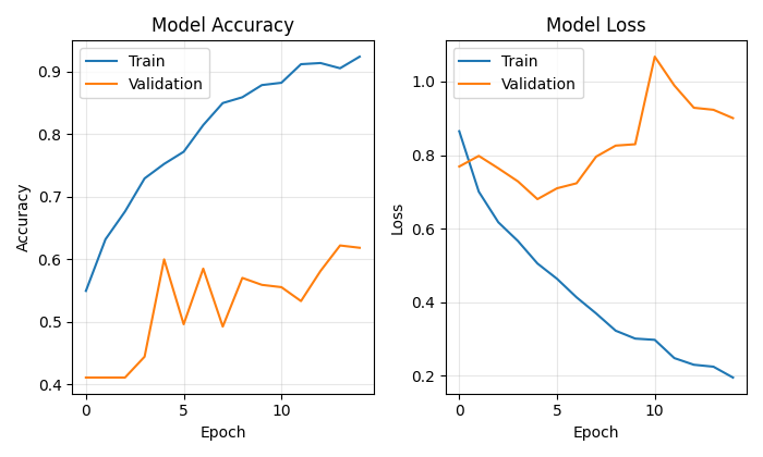
Training a model is not just about minimizing a loss function; it is a journey through the parameter landscape, where each iteration brings us closer to the goal:

# Early stopping to prevent overfitting
early_stopping = EarlyStopping(
    monitor='val_loss',
    patience=10,
    restore_best_weights=True,
    verbose=1
)

# Train model
history = model.fit(
    X_train, y_train,
    epochs=50,
    batch_size=32,
    validation_data=(X_val, y_val),
    callbacks=[early_stopping],
    verbose=1
)

We use Early Stopping to prevent overfitting - the neural network will stop learning when it stops improving on the validation set. This enables us to find the golden mean between underfitting and overfitting, the point of maximum generalization capability.

Looking into the consciousness of artificial intelligence

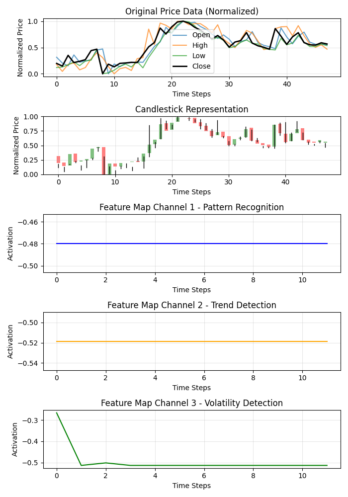
The uniqueness of our approach is the ability to visualize how the model "sees" the market. We have developed two special features that enable us to peer into the secrets of neural computing:

def visualize_model_perception(feature_model, last_window_scaled, window_size=48):
    # Get feature maps for the last window
    feature_maps = feature_model.predict(np.array([last_window_scaled]))[0]
    
    # Plot feature maps
    plt.figure(figsize=(7, 10))
    
    # Plot original data
    plt.subplot(5, 1, 1)
    plt.title("Original Price Data (Normalized)")
    plt.plot(np.arange(window_size), last_window_scaled[:, 0], label='Open', alpha=0.7)
    plt.plot(np.arange(window_size), last_window_scaled[:, 1], label='High', alpha=0.7)
    plt.plot(np.arange(window_size), last_window_scaled[:, 2], label='Low', alpha=0.7)
    plt.plot(np.arange(window_size), last_window_scaled[:, 3], label='Close', color='black', linewidth=2)
    
    # Plot candlestick representation
    plt.subplot(5, 1, 2)
    plt.title("Candlestick Representation")
    
    # Width of the candles
    width = 0.6
    
    for i in range(len(last_window_scaled)):
        # Candle color
        if last_window_scaled[i, 3] >= last_window_scaled[i, 0]:  # close >= open
            color = 'green'
            body_bottom = last_window_scaled[i, 0]  # open
            body_height = last_window_scaled[i, 3] - last_window_scaled[i, 0]  # close - open
        else:
            color = 'red'
            body_bottom = last_window_scaled[i, 3]  # close
            body_height = last_window_scaled[i, 0] - last_window_scaled[i, 3]  # open - close
        
        # Candle body
        plt.bar(i, body_height, bottom=body_bottom, color=color, width=width, alpha=0.5)
        
        # Candle wicks
        plt.plot([i, i], [last_window_scaled[i, 2], last_window_scaled[i, 1]], color='black', linewidth=1)
    
    # Plot feature maps visualization (first 3 channels)
    plt.subplot(5, 1, 3)
    plt.title("Feature Map Channel 1 - Pattern Recognition")
    plt.plot(time_indices, feature_maps[:, 0], color='blue')
    
    plt.subplot(5, 1, 4)
    plt.title("Feature Map Channel 2 - Trend Detection")
    plt.plot(time_indices, feature_maps[:, 1], color='orange')
    
    plt.subplot(5, 1, 5)
    plt.title("Feature Map Channel 3 - Volatility Detection")
    plt.plot(time_indices, feature_maps[:, 2], color='green')

This function creates a multi-panel visualization showing the original data, candlestick representation, and the activations of the first three channels of convolutional filters. Each channel specializes in a specific aspect of market dynamics: one captures recurring patterns, another one focuses on trends, and the third reacts to volatility. It's like uncovering the specialization of different areas of the experienced trader’s brain.

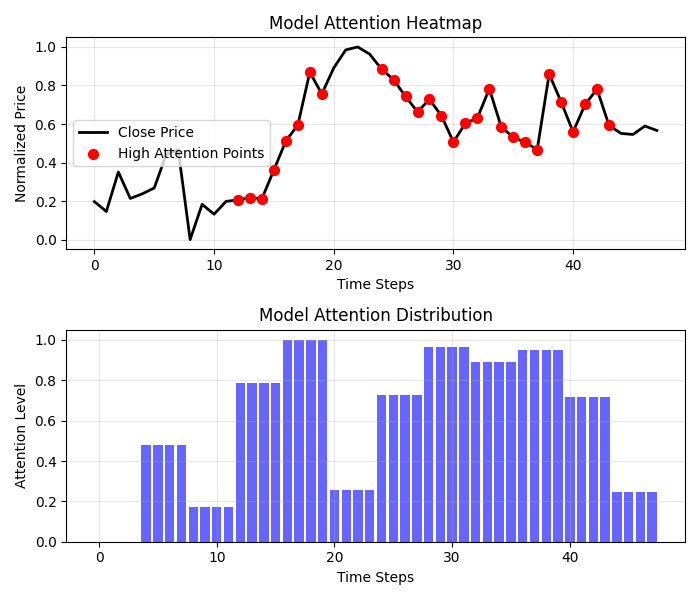
Even more exciting results are provided by the attention heatmap:

def visualize_attention_heatmap(feature_model, last_window_scaled, window_size=48):
    # Get feature maps for the last window
    feature_maps = feature_model.predict(np.array([last_window_scaled]))[0]
    
    # Average activation across all channels to get a measure of "attention"
    avg_activation = np.mean(np.abs(feature_maps), axis=1)
    
    # Normalize to [0, 1] for visualization
    attention = (avg_activation - np.min(avg_activation)) / (np.max(avg_activation) - np.min(avg_activation))
    
    # Upsample attention to match original window size
    upsampled_attention = np.zeros(window_size)
    ratio = window_size / len(attention)
    
    for i in range(len(attention)):
        start_idx = int(i * ratio)
        end_idx = int((i+1) * ratio)
        upsampled_attention[start_idx:end_idx] = attention[i]
    
    # Plot the heatmap
    plt.figure(figsize=(7, 6))
    
    # Price plot with attention heatmap
    plt.subplot(2, 1, 1)
    plt.title("Model Attention Heatmap")
    
    # Plot close prices
    time_indices = np.arange(window_size)
    plt.plot(time_indices, last_window_scaled[:, 3], color='black', linewidth=2, label='Close Price')
    
    # Add shading based on attention
    plt.fill_between(time_indices, last_window_scaled[:, 3].min(), last_window_scaled[:, 3].max(), 
                     alpha=upsampled_attention * 0.5, color='red')
                     
    # Highlight points with high attention
    high_attention_threshold = 0.7
    high_attention_indices = np.where(upsampled_attention > high_attention_threshold)[0]
    plt.scatter(high_attention_indices, last_window_scaled[high_attention_indices, 3], 
               color='red', s=50, zorder=5, label='High Attention Points')

This feature creates a real map of the model's consciousness, showing which areas of the chart it pays most attention to when making a decision. Red zones of increased attention often coincide with key levels and reversal points, confirming that our model has indeed learned to identify significant price formations.

From forecast to profit: Practical application

The final chord of our system is the visualization of the forecast and its presentation in a form understandable to the trader:

def plot_prediction(data, window_size=48, prediction_window=24, direction="UP ▲"):
    plt.figure(figsize=(7, 4.2))
    
    # Get the last window of data for visualization
    last_window = data.iloc[-window_size:]
    
    # Create time index for prediction
    last_date = last_window.index[-1]
    future_dates = pd.date_range(start=last_date, periods=prediction_window+1, freq=data.index.to_series().diff().mode()[0])[1:]
    
    # Plot closing prices
    plt.plot(last_window.index, last_window['close'], label='Historical Data')
    
    # Add marker for current price
    current_price = last_window['close'].iloc[-1]
    plt.scatter(last_window.index[-1], current_price, color='blue', s=100, zorder=5)
    plt.annotate(f'Current price: {current_price:.5f}', 
                 xy=(last_window.index[-1], current_price),
                 xytext=(10, -30),
                 textcoords='offset points',
                 fontsize=10,
                 arrowprops=dict(arrowstyle='->', color='black'))
    
    # Visualize the predicted direction
    arrow_start = (last_window.index[-1], current_price)
    
    # Calculate range for the arrow (approximately 10% of price range)
    price_range = last_window['high'].max() - last_window['low'].min()
    arrow_length = price_range * 0.1
    
    # Up or down prediction
    if direction == "UP ▲":
        arrow_end = (future_dates[-1], current_price + arrow_length)
        arrow_color = 'green'
    else:
        arrow_end = (future_dates[-1], current_price - arrow_length)
        arrow_color = 'red'
    
    # Direction arrow
    plt.annotate('', 
                 xy=arrow_end,
                 xytext=arrow_start,
                 arrowprops=dict(arrowstyle='->', lw=2, color=arrow_color))
    
    plt.title(f'EURUSD - Forecast for {prediction_window} periods: {direction}')

This visualization turns an abstract forecast into a clear trading signal. The green arrow indicates expected growth, the red one indicates a decline. A trader can instantly assess the current situation and make a decision supported by artificial intelligence analysis.

But our system goes beyond simply predicting direction. It provides a quantitative assessment of the confidence in the forecast:

# Predict on the last available window
def make_prediction(model, data, window_size=48):
    # Get the last window of data
    last_window = data.iloc[-window_size:][['open', 'high', 'low', 'close']]
    
    # Normalize data
    scaler = MinMaxScaler(feature_range=(0, 1))
    last_window_scaled = scaler.fit_transform(last_window)
    
    # Prepare data for the model
    last_window_reshaped = np.array([last_window_scaled])
    
    # Get prediction
    prediction = model.predict(last_window_reshaped)[0][0]
    
    # Interpret result
    direction = "UP ▲" if prediction > 0.5 else "DOWN ▼"
    confidence = prediction if prediction > 0.5 else 1 - prediction
    
    return direction, confidence * 100, last_window_scaled

The output value of the neural network is interpreted not just as a binary answer, but as the probability of an upward movement. This enables the trader to make informed decisions, taking into account not only the direction, but also system's confidence in its forecast. A forecast with 95% confidence may merit a more aggressive position than a forecast with 55% confidence.

Orchestrating process: The main function

All system elements are combined into the main function that coordinates the entire process from connecting to data to visualizing results:

def main():
    print("Starting EURUSD prediction system with computer vision")
    
    # Connect to MT5
    if not connect_to_mt5():
        return
    
    print("Successfully connected to MetaTrader5")
    
    # Load historical data
    bars_to_load = 2000  # Load more than needed for training
    data = get_historical_data(num_bars=bars_to_load)
    if data is None:
        mt5.shutdown()
        return
    
    print(f"Loaded {len(data)} bars of EURUSD history")
    
    # Convert data to image format
    print("Converting data for computer vision processing...")
    images, targets = create_images(data)
    print(f"Created {len(images)} images for training")
    
    # Train model
    print("Training computer vision model...")
    model, history, feature_model = train_cv_model(images, targets)
    
    # Visualize training process
    plot_learning_history(history)
    
    # Prediction
    direction, confidence, last_window_scaled = make_prediction(model, data)
    print(f"Forecast for the next 24 periods: {direction} (confidence: {confidence:.2f}%)")
    
    # Visualize prediction
    plot_prediction(data, direction=direction)
    
    # Visualize how the model "sees" the market
    visualize_model_perception(feature_model, last_window_scaled)
    
    # Visualize attention heatmap
    visualize_attention_heatmap(feature_model, last_window_scaled)
    
    # Disconnect from MT5
    mt5.shutdown()
    print("Work completed")

This function is like a conductor directing a complex symphony of data and algorithms. It takes us step by step through the entire process, from the first connection to the terminal to the final visualizations that reveal the inner world of artificial intelligence.

Conclusion: A new era of algorithmic trading

We have created something more than just another technical indicator or trading system. Our computer vision model is a new way of perceiving the market, a tool that enables us to look beyond human vision and discover patterns hidden in the noise of price movements.

It is not just a black box emitting signals of unknown origin. Thanks to visualizations, we can see how the model perceives the market, what features of price movement it pays attention to, and how its forecasts are formed. This creates a new level of trust and understanding between the trader and the algorithm.

In an era where high-frequency algorithms execute millions of trades per second, our system represents a different, more profound approach to algorithmic trading, an approach based not on execution speed, but on a deep understanding of market dynamics through the lens of computer vision.

The code is open, the technology is accessible, the results are impressive. Your journey into the world of computer vision for trading is just beginning. And who knows, perhaps this very perspective — through the algorithmic prism of neural networks — will enable you to see what previously remained invisible and find the key to understanding the ever-changing dance of currency quotations.

Imagine a trading session of the future: on your screen there are not only traditional candlestick charts and indicator lines, but also a live visualization of how artificial intelligence perceives the current market situation, what patterns it highlights, and what price levels it pays special attention to. This is not science fiction. It is technology available today. All that remains is to take a step towards a new era of algorithmic trading.