
Reimagining Classic Strategies (Part 21): Bollinger Bands And RSI Ensemble Strategy Discovery

The Bollinger Bands are a hallmark technical indicator used by traders across all levels of experience. They are most commonly employed to either identify support and resistance levels or they can also be used to facilitate mean-reverting trading strategies. The dominant belief underlying their use is that price levels tend to revert toward an equilibrium price level. The indicator is defined by a moving average that is enveloped by an upper and lower band, each set at a specified standard deviation above and below the moving average. The width of this standard deviation is an important tuning parameter of the indicator.
Under the classical setup, when price breaks above the upper Bollinger Band, it is anticipated that price will revert toward the central moving average. Conversely, when the price breaks below the lower band, a move up toward the equilibrium is expected. In practice, however, markets do not always behave within such well-defined boundaries. In some regimes, markets exhibit mean-reverting behavior, where the classical Bollinger Band setup can be profitable. During other regimes, markets follow strong trends, and traders relying on these classical rules may experience persistent losses. This raises the open-ended question of how Bollinger Bands can be used profitably despite constant shifts in market regime.
One possible solution is to pair Bollinger Bands with another technical indicator to help filter between mean-reverting moves and trending conditions. A strong candidate for this role is the Relative Strength Index (RSI). By coupling these two indicators, long trades are considered only when the price breaks below the lower extreme band and the RSI simultaneously enters oversold territory. This provides additional confirmation that price is likely to rally back toward equilibrium. Similarly, when the price breaks above the upper extreme band, short trades are considered only if the RSI also enters overbought regions, increasing the likelihood of a move back toward the mean.
This article explores the feasibility of the proposed coupling and outlines a process for refining the strategy. From our observations, we find that the Bollinger Bands and RSI do produce high-probability trading signals; however, these signals occur at a frequency that is too low to support systematic trading objectives. To address this limitation, five variations of the strategy are evaluated to extract additional signal while minimizing noise. While this process proved challenging, statistical modeling techniques allowed us to identify trading signals that were not immediately apparent through manually constructed rules. This article demonstrates how classical trading concepts can be adapted and extended using modern algorithmic approaches.
Important Information to Note
As we already stated in the introduction of our article, five versions of this trading strategy will be iteratively implemented. For readers that wish to follow along, we advise that you organize your application in the same structure that is denoted in Figure One below.

Figure 1: The file structure we will be following throughout this article
To avoid unnecessary repetition of the same information, we will now highlight important aspects of the backtest that we are going to conduct that will remain fixed across all five iterations of the application. We shall consider the first setting that we have to outline, which we will keep fixed, to be the time span of the backtest. Our backtest will run over three years, from January 2023 up until January 2026. All our backtests will be implemented on the EURUSD pair on the daily time frame.
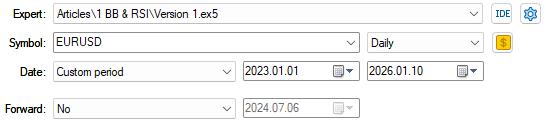
Figure 2: The backtest dates we will use across all 4 iterations of our applications
Additionally, we will use random delay settings to mimic the uncertainty of live trading. This gives us a realistic anticipation of the delays experienced when sending trades over real networks. Additionally, our modeling will be based on real ticks to ensure that the results we obtain are as close to reality as we can get while still depending on historical data.
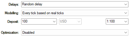
Figure 3: The backtest conditions denoted above will be fixed across all our tests
Establishing A Baseline
We shall begin by establishing a baseline version of our application to set profitability thresholds that we wish to outperform with all subsequent implementations of the application. The first order of business is to load the necessary trading libraries that we need for our application. We begin by loading the Trade library to help us manage our positions. Additionally, we will load a custom library called TradeInfo that we have written to help us manage tasks such as getting the current bid and ask prices and the minimum volume allowed on the market.//+------------------------------------------------------------------+ //| Version 1.mq5 | //| Copyright 2026, MetaQuotes Ltd. | //| https://www.mql5.com | //+------------------------------------------------------------------+ #property copyright "Copyright 2026, MetaQuotes Ltd." #property link "https://www.mql5.com" #property version "1.00" //+------------------------------------------------------------------+ //| Libraries | //+------------------------------------------------------------------+ #include <Trade/Trade.mqh> #include <VolatilityDoctor/Trade/TradeInfo.mqh> CTrade Trade; TradeInfo *TradeHelper;
With that established, the next important step for us to take is to now define important system constants that must be held consistently throughout all iterations of our application. These system definitions are important tuning parameters of our trading strategy, and changing these system definitions will drastically change the performance of the trading strategy. Therefore, to ensure that all the improvements that we will observe are coming from improvements being made to our trading logic, it is paramount that we fix these important tuning parameters.
//+------------------------------------------------------------------+
//| System definitions                                               |
//+------------------------------------------------------------------+
#define ATR_PERIOD    14
#define ATR_MULTIPLE  2
#define BB_PERIOD     30
#define BB_SD         2
#define BB_PRICE      PRICE_CLOSE
#define RSI_PERIOD    15
#define RSI_PRICE     PRICE_CLOSE
#define RSI_LEVEL_MAX 70
#define RSI_LEVEL_MIN 30
#define SYMBOL        "EURUSD"
#define TF_MAIN       PERIOD_D1
#define TF_TRADING    PERIOD_H4
#define SHIFT         0
Once we have set up our tuning parameters, we now define global variables that will be used in numerous different scopes throughout our trading application. These global variables constitute the handlers and the buffers of our technical indicators.
//+------------------------------------------------------------------+
//| Global Variables                                                 |
//+------------------------------------------------------------------+
int      bb_handler,rsi_handler,atr_handler;
double   bb_upper[],bb_mid[],bb_lower[],rsi[],atr[];
When our trading application is initialized for the first time, we begin by first defining our indicator handlers. After loading the appropriate technical indicators, our next order of business is to ensure that each of our technical indicators has been loaded correctly and that none of them are invalid. We do this by simply checking if each handle is equal to the `INVALID_HANDLE` macro that is defined in the MQL5 API. If any of the indicators fail to load correctly, we will give the user feedback and then terminate the initialization process. Otherwise, if all is well, we will load our custom-defined class and return a successful initialization.
//+------------------------------------------------------------------+
//| Expert initialization function                                   |
//+------------------------------------------------------------------+
int OnInit()
  {
//--- Setup the technical indicators
   bb_handler  = iBands(SYMBOL,TF_MAIN,BB_PERIOD,SHIFT,BB_SD,BB_PRICE);
   rsi_handler = iRSI(SYMBOL,TF_MAIN,RSI_PERIOD,RSI_PRICE);
   atr_handler = iATR(SYMBOL,TF_MAIN,ATR_PERIOD);

//--- Validate the indicators were setup correctly
   if(bb_handler == INVALID_HANDLE)
     {
      //--- Failed to sertup the Bollinger Bands
      Comment("Failed to setup the Bollinger Bands Indicator: ",GetLastError());
      return(INIT_FAILED);
     }

   else
      if(rsi_handler == INVALID_HANDLE)
        {
         //--- Failed to setup the RSI indicator
         Comment("Failed to setup the RSI Indicator: ",GetLastError());
         return(INIT_FAILED);
        }

      else
         if(atr_handler == INVALID_HANDLE)
           {
            //--- Failed to setup the ATR indicator
            Comment("Failed to setup the ATR Indicator: ",GetLastError());
            return(INIT_FAILED);
           }

         else
           {
            //--- User defined types
            TradeHelper = new TradeInfo(SYMBOL,TF_MAIN);

            //--- Good news: no errors
            return(INIT_SUCCEEDED);

           }
  }
When our application is no longer in use, we will release the memory resources that the terminal allocated for the indicators and the library that we loaded. This is good programming practice in MQL5, as it ensures that we clean up after ourselves.
//+------------------------------------------------------------------+
//| Expert deinitialization function                                 |
//+------------------------------------------------------------------+
void OnDeinit(const int reason)
  {
//--- Release the indicators
   IndicatorRelease(bb_handler);
   IndicatorRelease(rsi_handler);
   IndicatorRelease(atr_handler);
   delete TradeHelper;
  }
Whenever new price levels are received from the broker, we begin by keeping track of time. In MQL5, it is easy to algorithmically detect the formation of a new candle. If a new candle has formed, we update our last recorded timestamp and proceed to update our indicator buffers. Lastly, before we check our trading rules, we also keep track of the closing price.
We only allow our application to open one position at a time. Therefore, we begin by checking if we have zero positions open. If this is the case, then we trade according to the rules described in the introduction of the article. That is to say, if the closing price is above the uppermost extreme Bollinger Band and the RSI is in the overbought region, then we will sell. The converse is true for long positions: we wait for price to break beneath the lowest Bollinger Band and for the RSI to enter oversold regions.
//+------------------------------------------------------------------+
//| Expert tick function                                             |
//+------------------------------------------------------------------+
void OnTick()
  {
//--- Keep track of the time
   static datetime time_stamp;
   datetime time_current = iTime(SYMBOL,TF_TRADING,0);

//--- Check if a new candle has formed
   if(time_stamp != time_current)
     {
      //--- Update the time
      time_stamp = time_current;

      //--- Update our indicator readings
      CopyBuffer(bb_handler,0,0,1,bb_mid);
      CopyBuffer(bb_handler,1,0,1,bb_upper);
      CopyBuffer(bb_handler,2,0,1,bb_lower);
      CopyBuffer(rsi_handler,0,0,1,rsi);
      CopyBuffer(atr_handler,0,0,1,atr);

      //--- Update current price levels
      double close = iClose(SYMBOL,TF_MAIN,SHIFT);

      //--- If we have no open positions
      if(PositionsTotal() == 0)
        {
         //--- Check for our trading signal
         if((close > bb_upper[0]) && (rsi[0] > RSI_LEVEL_MAX))
           {
            Trade.Sell(TradeHelper.MinVolume(),TradeHelper.GetSymbol(),TradeHelper.GetBid(),TradeHelper.GetBid() + (atr[0] * ATR_MULTIPLE),TradeHelper.GetBid() - (atr[0] * ATR_MULTIPLE),"");
           }

         else
            if((close < bb_lower[0]) && (rsi[0] < RSI_LEVEL_MIN))
              {
               Trade.Buy(TradeHelper.MinVolume(),TradeHelper.GetSymbol(),TradeHelper.GetAsk(),TradeHelper.GetAsk() - (atr[0] * ATR_MULTIPLE),TradeHelper.GetAsk() + (atr[0] * ATR_MULTIPLE),"");
              }
        }
     }
  }
//+------------------------------------------------------------------+
This concludes our application. The final step is to undefine all the system definitions that we entered in the header of the application. Again, this is another good programming practice in MQL5.
//+------------------------------------------------------------------+
//| Undefine system constants                                        |
//+------------------------------------------------------------------+
#undef ATR_PERIOD
#undef ATR_MULTIPLE
#undef BB_PERIOD
#undef BB_SD
#undef BB_PRICE
#undef RSI_PERIOD
#undef RSI_PRICE
#undef SYMBOL
#undef TF_MAIN
#undef SHIFT
#undef TF_TRADING
//+------------------------------------------------------------------+
The equity curve produced by the trading rules we have defined is depicted for the reader below in Figure 4. As we can see, the equity curve exhibits an upward trend. Although it does experience drawdown periods and some unacceptable levels of volatility, the overall trend is positive.
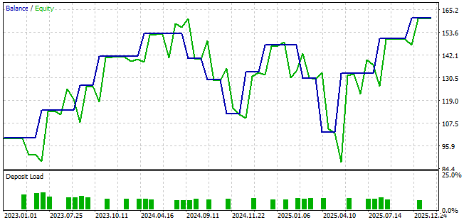
Figure 4: The equity curve produced by our initial attempt to combine the Bollinger Bands and the RSI
When we analyze the detailed statistics of the trading rules we have defined, we observe a mixed set of positive and negative results. We begin with the positive aspects of the trading strategy. We observe that 64% of all trades placed by the rules were profitable. This represents pristine quality, high-quality trading signals, and the expected payoff is 4.37. These statistics are very encouraging.
However, the total number of trades placed was only 14. The reader should recall that this backtest ran over a period of three years. This means that, on average, fewer than five trades were placed per year. This is dismal and unacceptable on any level. Therefore, we wish to intelligently discover more signal and unearth additional trading opportunities without deteriorating the quality of the strategy. This is a delicate balance to strike, and the appropriate rules to follow are not immediately obvious.
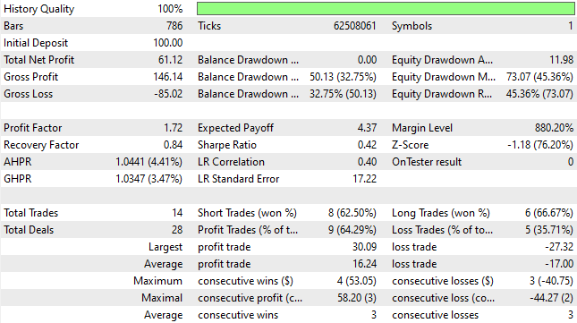
Figure 5: The detailed statistics produced by our first iteration of our trading application
Improving The Baseline
In an attempt to improve our initial performance levels, we tried many different handwritten rules to improve both the signal-to-noise ratio and the frequency of trades. Our intuition suggested that by looking for strong momentum in the market, we might be able to unearth high-quality trading opportunities. Many fundamental traders use candlestick patterns to analyze market sentiment. Therefore, we searched for candlestick patterns that indicate strong market movement.//--- Update current price levels double close = iClose(SYMBOL,TF_MAIN,SHIFT); double open_current = iOpen(SYMBOL,TF_MAIN,SHIFT); double open_previous = iOpen(SYMBOL,TF_MAIN,1); double low_current = iLow(SYMBOL,TF_MAIN,SHIFT); double low_previous = iLow(SYMBOL,TF_MAIN,1); double high_current = iHigh(SYMBOL,TF_MAIN,SHIFT); double high_previous = iHigh(SYMBOL,TF_MAIN,1);
One commonly cited rule that traders abide by is the identification of higher highs or lower lows. If the highest price of the current day is higher than the highest price of the previous day, this indicates a strong upward price movement. Conversely, if the lowest price of the current day is lower than the lowest price of the previous day, this indicates strong downward momentum. We therefore believed that coupling these two trading strategies could refine our entries and provide more reliable trading opportunities.
//--- If we have no open positions
if(PositionsTotal() == 0)
        {
         //--- Check for our trading signal
         if(((close > bb_upper[0]) && (rsi[0] > RSI_LEVEL_MAX)) || ((low_current<low_previous) && (high_current>high_previous) && (open_current<open_previous) && (close < bb_mid[0])))
           {
            Trade.Sell(TradeHelper.MinVolume(),TradeHelper.GetSymbol(),TradeHelper.GetBid(),TradeHelper.GetBid() + (atr[0] * ATR_MULTIPLE),TradeHelper.GetBid() - (atr[0] * ATR_MULTIPLE),"");
           }

         else
            if(((close < bb_lower[0]) && (rsi[0] < RSI_LEVEL_MIN)) || ((high_current>high_previous) && (low_current<low_previous) && (open_current>open_previous) && (close > bb_mid[0])))
              {
               Trade.Buy(TradeHelper.MinVolume(),TradeHelper.GetSymbol(),TradeHelper.GetAsk(),TradeHelper.GetAsk() - (atr[0] * ATR_MULTIPLE),TradeHelper.GetAsk() + (atr[0] * ATR_MULTIPLE),"");
              }
        }
However, as the reader can see from the resulting equity curve, although the strategy was profitable, it failed to meet our expectations. The new trading strategy reached balance levels lower than any previously observed. In the initial setup, the strategy reached a low of $84, whereas in the current setup it reached a new low of $71. This is undesirable.
Additionally, the final balance of the initial trading strategy exceeded $150, whereas the new strategy concluded below $140. As a result, nothing observed in the equity curve encourages continued use of the new rules that our intuition suggested would work.
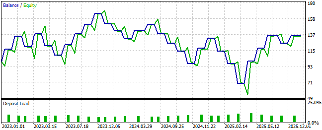
Figure 6: The equity curve produced by the second iteration of our Expert Advisor failed to meet our expectations
When analyzing the detailed statistics of the new trading strategy, we observe that the total number of trades increased to 29 from an initial total of 14. This represents a 100% improvement and confirms that we succeeded in uncovering additional signal. However, the total net profit declined from $61 to $35, indicating that additional noise was introduced into the strategy. Although the strategy remained profitable, it cannot be considered a success relative to the benchmark performance.
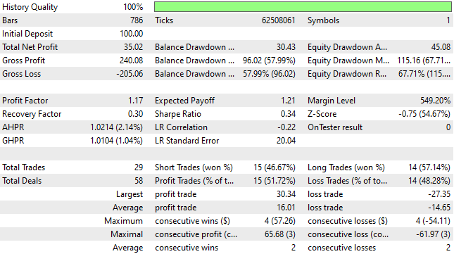
Figure 7: The detailed statistics produced by the second iteration of our trading application reveal deep flaws in our trading logic
Fetching Historical Market Data
Although only two versions of the trading strategy were depicted, the reader should rest assured that many additional iterations were tested. After exhausting manual rule-based approaches, we concluded that leveraging statistical models could help us discover trading rules beyond what intuition alone could produce. To accomplish this, we first wrote a script to extract historical data from the terminal into a CSV file. Using the same system definitions as before, we wrote the historical open, high, low, close, and technical indicator values to disk.//+------------------------------------------------------------------+ //| Fetch Data Bollinger Bands RSI Strategy | //| Copyright 2026, CompanyName | //| http://www.companyname.net | //+------------------------------------------------------------------+ #property copyright "Copyright 2026, MetaQuotes Ltd." #property link "https://www.mql5.com" #property version "1.00" #property script_show_inputs //+------------------------------------------------------------------+ //| System definitions | //+------------------------------------------------------------------+ #define BB_PERIOD 30 #define BB_SD 2 #define BB_PRICE PRICE_CLOSE #define RSI_PERIOD 15 #define RSI_PRICE PRICE_CLOSE #define RSI_LEVEL_MAX 70 #define RSI_LEVEL_MIN 30 #define TF_MAIN PERIOD_D1 #define SHIFT 0 //+------------------------------------------------------------------+ //| Global Variables | //+------------------------------------------------------------------+ double bb_upper[],bb_mid[],bb_lower[],rsi[]; //--- Setup the technical indicators int bb_handler = iBands(Symbol(),TF_MAIN,BB_PERIOD,SHIFT,BB_SD,BB_PRICE); int rsi_handler = iRSI(Symbol(),TF_MAIN,RSI_PERIOD,RSI_PRICE); //--- File name string file_name = Symbol() + " Bollinger Band RSI Data.csv"; //--- Amount of data requested input int size = 365; //+------------------------------------------------------------------+ //| Our script execution | //+------------------------------------------------------------------+ void OnStart() { //--- Write to file int file_handle=FileOpen(file_name,FILE_WRITE|FILE_ANSI|FILE_CSV,","); CopyBuffer(bb_handler,0,0,size,bb_mid); ArraySetAsSeries(bb_mid,true); CopyBuffer(bb_handler,1,0,size,bb_upper); ArraySetAsSeries(bb_upper,true); CopyBuffer(bb_handler,2,0,size,bb_lower); ArraySetAsSeries(bb_lower,true); CopyBuffer(rsi_handler,0,0,size,rsi); ArraySetAsSeries(rsi,true); for(int i=size;i>=1;i--) { if(i == size) { FileWrite(file_handle, //--- Time "Time", //--- OHLC "Open", "High", "Low", "Close", //--- Technical Indicators "BB Upper", "BB Mid", "BB Lower", "RSI" ); } else { FileWrite(file_handle, iTime(_Symbol,PERIOD_CURRENT,i), //--- OHLC iOpen(_Symbol,PERIOD_CURRENT,i), iHigh(_Symbol,PERIOD_CURRENT,i), iLow(_Symbol,PERIOD_CURRENT,i), iClose(_Symbol,PERIOD_CURRENT,i), //--- Technical Indicators bb_upper[i], bb_mid[i], bb_lower[i], rsi[i] ); } } //--- Close the file FileClose(file_handle); } //+------------------------------------------------------------------+
Reaching New Performance Levels
Once saved, the data was analyzed using statistical libraries in Python. The first step involved loading the required analytical libraries, followed by reading the CSV file generated by the MQL5 script.
#Load the analytical libraries
import pandas as pd
import numpy as np
import seaborn as sns
import matplotlib.pyplot as plt
To avoid data leakage, we ensured that the AI model was not trained on the same dates used for backtesting. The three-year backtest period was therefore removed from the training set.
#Read in the data
data = pd.read_csv("/ENTER/YOUR/PATH/HERE/EURUSD Bollinger Band RSI Data.csv")
A snapshot of the resulting training data was provided for reference.
#Drop the dates that overlap with our backtest
train = data.iloc[:((-365 * 2) - 90),:]
test  = data.iloc[((-365 * 2) - 90):,:]

#Check the dates left
train
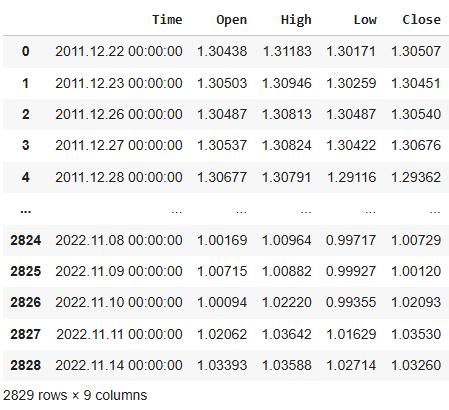
Figure 8: We have filtered out all the observations that overlap with our backtest period. Be sure to do the same for best practice.
To validate the correctness of the exported data, we plotted the values. As shown, the Bollinger Bands correctly envelop price, confirming that the data was written correctly.
plt.plot(data['Close'],color='green')
plt.plot(data['BB Upper'],color='red')
plt.plot(data['BB Lower'],color='blue')
plt.grid()
plt.title('Visualizing Historical EURUSD Exchange Rates')
plt.ylabel('Exchange Rate')
plt.xlabel('Historical Time')
plt.legend(['EURUSD Close','BB Upper','BB Lower'])
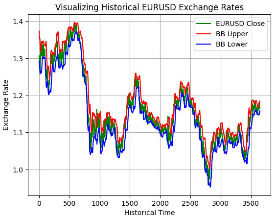
Figure 9: Visually inspecting if our MQL5 script correctly captured the intended historical EURUSD data
Because it is not immediately obvious which statistical model will perform best, we evaluated multiple candidate models using cross-validation.
#Load our machine learning training libraries
from sklearn.linear_model import LinearRegression,Ridge,Lasso,ARDRegression
from sklearn.neighbors    import KNeighborsRegressor,RadiusNeighborsRegressor
from sklearn.svm          import LinearSVR
from sklearn.ensemble     import RandomForestRegressor,BaggingRegressor,AdaBoostRegressor
from sklearn.model_selection import TimeSeriesSplit,cross_val_score
We defined the forecast horizon.
#Define our forecast horizon
HORIZON = 5
And then labeled the data using the future closing price.
#Label the data
train['Target'] = train['Close'].shift(-HORIZON)
A dictionary of candidate models was created.
#List all the models we wish to evaluate
models = [LinearRegression(),Ridge(),Lasso(),ARDRegression(),KNeighborsRegressor(),RadiusNeighborsRegressor(),LinearSVR(),RandomForestRegressor(),BaggingRegressor(),AdaBoostRegressor()]
Their performance was evaluated using time-series cross-validation. Because shuffling observations is unacceptable for time-series forecasting, we used the `TimeSeriesSplit` object from the scikit-learn library.
#Define a time series cross validation object
tscv = TimeSeriesSplit(
  n_splits=5,
  gap=HORIZON
)
We will now prepare to store the performance levels achieved by each model we selected from our machine learning library.
#Store the performance of each model
scores = []
Each model’s mean squared error was calculated and recorded.
#Evaluate each model
for model in models:
  #User feedback
  print("Evaluating model: ",model)
  #Store the current score
  current_score = np.mean(np.abs(cross_val_score(model,train.iloc[:,1:-1],train.iloc[:,-1],cv=tscv,scoring='neg_mean_squared_error')))
  scores.append(current_score)
Upon visualizing the results, model 3 emerged as the best performer. Although model 5 appeared to produce near-zero error, it failed cross-validation and returned NaN values. This information has been provided in detail for the reader in the table that follows.
sns.barplot(scores)
plt.ylabel('Cross Validated RMSE')
plt.xlabel('Model')
plt.title('Model Selection For The EURUSD Market')
plt.axhline(scores[3],linestyle=':',color='red') 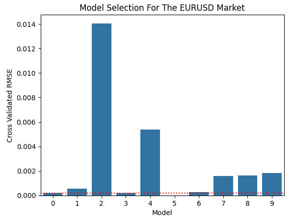
Figure 10: The ARDRegression model was the best-performing model we identified in this exercise
Model 3 corresponds to the ARD Regressor. Therefore, we will prepare to export this model to ONNX format.
| Model | Error |
|---|---|
| Linear Regression | 0.0001957533746919363 |
| Ridge | 0.000550907245398377 |
| Lasso | 0.014059369238373157 |
| ARDRegression | 0.00018190369036281064 |
| KNeighborsRegressor | 0.005387854064255319 |
| RadiusNeighborsRegressor | nan |
| LinearSVR | 0.0002872914823846638 |
| RandomForestRegressor | 0.0015833296216492855 |
| BaggingRegressor | 0.0016147744161974461 |
| AdaBoostRegressor | 0.0018082307134142561 |
Exporting Our Model To ONNX Format
The ARD model was exported using the ONNX library. The Open Neural Network Exchange (ONNX) library allows machine learning models to be deployed in a language-agnostic format, making it easier for developers to rapidly prototype and deploy machine learning models of any complexity.
import onnx
from skl2onnx.common.data_types import FloatTensorType
from skl2onnx import convert_sklearn
The model input shape was defined as one by eight floats.
initial_types = [('float_input',FloatTensorType([1,8]))]
Our ARD model was then fit on the full training set.
model = ARDRegression()
model.fit(train.iloc[:,1:-1],train.iloc[:,-1])
Next, we converted the model to its ONNX prototype.
onnx_proto = convert_sklearn(model,initial_types=initial_types,target_opset=12) And finally, we saved the ONNX file to disk.
onnx.save(onnx_proto,"EURUSD D1 ARDRegression.onnx") Implementing Our Suggested Improvements
The ONNX model we exported from Python, was then loaded into the Expert Advisor as a resource.
//+------------------------------------------------------------------+
//| System resources                                                 |
//+------------------------------------------------------------------+
#resource "\\Files\\EURUSD D1 ARDRegression.onnx" as const uchar onnx_buffer[];
Additionally, new system definitions were introduced to define the model’s input and output dimensions.
#define ONNX_INPUTS   8
#define ONNX_OUTPUTS  1
That is not all we must do; we must also consider new global variables for the model and its predictions.
long     onnx_model;
vectorf  onnx_outputs;
During initialization, the model’s input and output shapes were validated. If validation failed, initialization was aborted and feedback was provided. Otherwise, the model outputs were initialized to zero.
//+------------------------------------------------------------------+
//| Expert initialization function                                   |
//+------------------------------------------------------------------+
int OnInit()
  {

//--- Set up the ONNX model
   onnx_model = OnnxCreateFromBuffer(onnx_buffer,ONNX_DATA_TYPE_FLOAT);

//--- Define the model I/O shapes
   ulong onnx_input_shape[] = {1,ONNX_INPUTS};
   ulong onnx_output_shape[] = {1,ONNX_OUTPUTS};

//--- Validate the ONNX model
   else
      if(!OnnxSetInputShape(onnx_model,0,onnx_input_shape))
        {
         Comment("Failed to define the ONNX model input shape: ",GetLastError());
         return(INIT_FAILED);
        }

      else
         if(!OnnxSetOutputShape(onnx_model,0,onnx_output_shape))
           {
            Comment("Failed to define the ONNX model output shape: ",GetLastError());
            return(INIT_FAILED);
           }

         else
            if(onnx_model == INVALID_HANDLE)
              {
               Comment("Error occured setting up the ONNX model: ",GetLastError());
               return(INIT_FAILED);
              }

            //--- Final settings
            else
              {
              //--- Initialize the ONNX model outputs with a zero
              onnx_outputs = vectorf::Zeros(ONNX_OUTPUTS);

               //--- Good news: no errors
               return(INIT_SUCCEEDED);
              }
  }
When the application terminates, the ONNX model and allocated resources are released, and the terminal comments are cleared.
//+------------------------------------------------------------------+
//| Expert deinitialization function                                 |
//+------------------------------------------------------------------+
void OnDeinit(const int reason)
  {
   OnnxRelease(onnx_model);
   Comment("");
  }
When new price data arrives, model inputs are stored as floats, and predictions are generated using the ONNX runtime. Trades may be opened based on the model’s forecasted direction.
//+------------------------------------------------------------------+
//| Expert tick function                                             |
//+------------------------------------------------------------------+
void OnTick()
  {

//--- Check if a new candle has formed
   if(time_stamp != time_current)
     {

      //--- Prepare our ONNX model inputs
      vectorf onnx_inputs = {(float)iOpen(SYMBOL,TF_MAIN,SHIFT),
                             (float)iHigh(SYMBOL,TF_MAIN,SHIFT),
                             (float)iLow(SYMBOL,TF_MAIN,SHIFT),
                             (float)iClose(SYMBOL,TF_MAIN,SHIFT),
                             (float)bb_upper[0],
                             (float)bb_mid[0],
                             (float)bb_lower[0],
                             (float)rsi[0]};

      //--- Obtain a forecast from our ONNX model
      OnnxRun(onnx_model,ONNX_DATA_TYPE_FLOAT,onnx_inputs,onnx_outputs);
      Comment("EURUSD Model Forecast: ",onnx_outputs[0]);

      //--- If we have no open positions
      if(PositionsTotal() == 0)
        {
         //--- Check for our trading signal
         if(((close > bb_upper[0]) && (rsi[0] > RSI_LEVEL_MAX)) || (onnx_outputs[0] < close))
           {
            Trade.Sell(TradeHelper.MinVolume(),TradeHelper.GetSymbol(),TradeHelper.GetBid(),TradeHelper.GetBid() + (atr[0] * ATR_MULTIPLE),TradeHelper.GetBid() - (atr[0] * ATR_MULTIPLE),"");
           }

         else
            if(((close < bb_lower[0]) && (rsi[0] < RSI_LEVEL_MIN)) || (onnx_outputs[0] > close))
              {
               Trade.Buy(TradeHelper.MinVolume(),TradeHelper.GetSymbol(),TradeHelper.GetAsk(),TradeHelper.GetAsk() - (atr[0] * ATR_MULTIPLE),TradeHelper.GetAsk() + (atr[0] * ATR_MULTIPLE),"");
              }
        }
     }
  }
//+------------------------------------------------------------------+
Always remember to undefine all system constants at the end of your application.
//+------------------------------------------------------------------+
//| Undefine system constants                                        |
//+------------------------------------------------------------------+
#undef ONNX_INPUTS
#undef ONNX_OUTPUTS
//+------------------------------------------------------------------+
Unfortunately, the resulting equity curve revealed a further deterioration in performance.

Figure 11: The equity curve obtained by the third iteration of our Expert Advisor challenges us to be more diligent with our methodology
Net profit reached an all-time low of $6, indicating excessive noise despite increased trade frequency.

Figure 12: Our detailed statistics clearly suggest that no improvements have been realized by the changes we have proposed so far
Digging Deeper For Better Performance
Due to the poor performance we observed, we had to revise our modeling approach from the ground up. In our previous discussion on statistical modeling of financial markets, we empirically observed that we can obtain higher accuracy levels when we model certain technical indicators instead of modeling raw price levels directly; a link to that article has been provided here for the reader's convenience. As a result, we shifted focus from predicting price directly to instead forecasting the technical indicators involved in our trading strategy.#Label the data train['Target 1'] = train['BB Upper'].shift(-HORIZON) train['Target 2'] = train['BB Mid'].shift(-HORIZON) train['Target 3'] = train['BB Lower'].shift(-HORIZON) train['Target 4'] = train['RSI'].shift(-HORIZON) #Drop missing labels train = train.iloc[:-HORIZON,:]
The new model produced four outputs instead of one.
final_types = [('float_output',FloatTensorType([1,4]))]Additionally, we took the time to be more diligent to reduce the noise in our system. We achieved this end by applying Z-score normalization to scale the data accordingly.
Z1 = train.iloc[:,1:-4].mean()
Z2 = train.iloc[:,1:-4].std()
train.iloc[:,1:-4] = ((train.iloc[:,1:-4] - Z1) / Z2)
Because the ARD model appeared to underfit, we selected a Random Forest Regressor to capture nonlinear relationships.
model = RandomForestRegressor()

model.fit(train.iloc[:,1:-4],train.iloc[:,-4:])
The model was converted to ONNX, saved with descriptive naming conventions.
onnx_proto = convert_sklearn(model,initial_types=initial_types,final_types=final_types,target_opset=12)
onnx.save(onnx_proto,"EURUSD D1 RandomForestRegressor.onnx")
Implementing Improvements
From there we reloaded the new ONNX model into the application.//+------------------------------------------------------------------+ //| Version 4.mq5 | //| Copyright 2026, MetaQuotes Ltd. | //| https://www.mql5.com | //+------------------------------------------------------------------+ #property copyright "Copyright 2026, MetaQuotes Ltd." #property link "https://www.mql5.com" #property version "1.00" //+------------------------------------------------------------------+ //| System resources | //+------------------------------------------------------------------+ #resource "\\Files\\EURUSD D1 RandomForestRegressor.onnx" as const uchar onnx_buffer[];
The mean and standard deviation values we obtained in our Python analysis of historical market data were carefully stored as floats to prevent truncation.
//+------------------------------------------------------------------+
//| System constants                                                 |
//+------------------------------------------------------------------+
//--- Column Mean Values
const float Z1[] = { (float)1.18132371,  (float)1.18577335,  (float)1.17706596,  (float)1.1812953 ,  (float)1.20514458,
                     (float)1.18303579,  (float)1.16092701,  (float)48.60276562};

//--- Column Standard Deviation
const float Z2[] = { (float)0.09684736,  (float)0.09665192,  (float)0.09686825,  (float)0.09684589,  (float)0.09614994,
                     (float)0.09556366,  (float)0.09612185,  (float)11.10783131};
All our inputs were scaled before inference to ensure that our model is not overfitting to noise caused by differences in scale. And, new trading rules were introduced that combined forecasted RSI direction and the forecasted slope of the middle Bollinger Band with the original trading signal we started with.
//+------------------------------------------------------------------+
//| Expert tick function                                             |
//+------------------------------------------------------------------+
void OnTick()
  {

//--- Check if a new candle has formed
   if(time_stamp != time_current)
     {
      //--- Update the time
      time_stamp = time_current;

      //--- Prepare our ONNX model inputs
      vectorf onnx_inputs = {(float)iOpen(SYMBOL,TF_MAIN,SHIFT),
                             (float)iHigh(SYMBOL,TF_MAIN,SHIFT),
                             (float)iLow(SYMBOL,TF_MAIN,SHIFT),
                             (float)iClose(SYMBOL,TF_MAIN,SHIFT),
                             (float)bb_upper[0],
                             (float)bb_mid[0],
                             (float)bb_lower[0],
                             (float)rsi[0]};

      //--- Scale the model inputs appropriately
      for(int i = 0; i < ONNX_INPUTS;i++)
         {
            onnx_inputs[i] = ((onnx_inputs[i]-Z1[i])/Z2[i]);
         }

      //--- Obtain a forecast from our ONNX model
      OnnxRun(onnx_model,ONNX_DATA_TYPE_FLOAT,onnx_inputs,onnx_outputs);
      Comment("EURUSD Model Forecast: ",onnx_outputs);

      //--- If we have no open positions
      if(PositionsTotal() == 0)
        {
         //--- Check for our trading signal
         if(((close > bb_upper[0]) && (rsi[0] > RSI_LEVEL_MAX)) || ((onnx_outputs[3] < rsi[0]) && (onnx_outputs[1] < bb_mid[0])))
           {
            Trade.Sell(TradeHelper.MinVolume(),TradeHelper.GetSymbol(),TradeHelper.GetBid(),TradeHelper.GetBid() + (atr[0] * ATR_MULTIPLE),TradeHelper.GetBid() - (atr[0] * ATR_MULTIPLE),"");
           }

         else
            if(((close < bb_lower[0]) && (rsi[0] < RSI_LEVEL_MIN)) || ((onnx_outputs[3] > rsi[0]) && (onnx_outputs[1] > bb_mid[0])))
              {
               Trade.Buy(TradeHelper.MinVolume(),TradeHelper.GetSymbol(),TradeHelper.GetAsk(),TradeHelper.GetAsk() - (atr[0] * ATR_MULTIPLE),TradeHelper.GetAsk() + (atr[0] * ATR_MULTIPLE),"");
              }
        }
     }
  }
//+------------------------------------------------------------------+
The resulting equity curve demonstrated significant improvement, reaching new highs near $300 while maintaining higher minimum equity levels.

Figure 13: The equity curve produced by our fourth iteration of the trading application finally yields the results we desire to observe
Total trades increased to 78, and net profit rose to $95. Although the win rate declined from 64% to 55%, both objectives—higher trade frequency and higher profitability—were achieved.

Figure 14: Our detailed statistics have improved materially over the benchmark performance levels we established
Analyzing Our Improvements
In most of our discussions, we employ statistical libraries to perform inference on market data. However, modern statistical libraries enable far more than inference alone; they also allow us to analyze data in ways that expose and explain the underlying structure of the market.
We therefore begin by assessing whether the relationship we believe exists between the RSI and future price action actually holds. To investigate this, we constructed a scatter plot of the closing price against the RSI reading. Each data point was colored blue if price action was bearish and orange if price action was bullish. A red line was plotted to generalize the region in which RSI readings are considered overbought, thereby triggering sell orders, while a green line demarcated the oversold region where long positions would be entered.
Under our expectations, we would observe a natural boundary that cleanly separates bullish and bearish samples. Instead, we observe a mixture of price action above and below the expected regions. This clearly indicates the presence of unmitigated noise in the trading signals generated by the RSI.
sns.scatterplot(data=train,x='Close',y='RSI',hue='Bin Target Threshold Price')
plt.axhline(data['RSI'].mean()+data['RSI'].std(),color='red')
plt.axhline(data['RSI'].mean()-data['RSI'].std(),color='green')
plt.grid()
plt.ylabel('RSI Reading')
plt.xlabel('EURUSD Close Price')
plt.title('Relationship Between RSI & EURUSD Return')
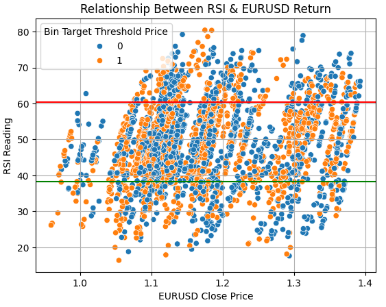
Figure 15: The RSI indicator fails to naturally discriminate bullish and bearish price action
We extended the same analysis to trading signals generated by the Bollinger Bands. We began by analyzing the difference between the upper band and the closing price, plotting this against historical time. Points above the red line indicate that price has broken above the upper band. In this region, we would expect to observe only bearish samples. Instead, we again observe a mixture of bullish and bearish outcomes, indicating that price may either revert to the mean or continue trending upward. That said, the ratio of bearish to bullish samples is notably stronger for the Bollinger Band than what we observed for the RSI.
sns.scatterplot(data=train,y=train['Close']-train['BB Upper'],x=np.arange(train.shape[0]),hue='Bin Target Threshold Price')
plt.grid()
plt.axhline(0,color='red')
plt.ylabel('Difference Between Price & BB Upper')
plt.xlabel('Historical Time')
plt.title('Relationship Between EURUSD Close & BB Upper')
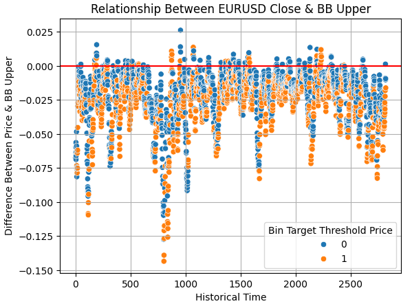
Figure 16: The Upper Bollinger Band appears to set a better decision boundary for us than the RSI
The same behavior is observed for the lower Bollinger Band. When the price breaks below the lower band, we expect to enter long positions. While it is encouraging that most samples below the green line are bullish, the continued presence of mixed outcomes confirms that none of the technical indicators considered perfectly discriminate between bullish and bearish price action. Nevertheless, the Bollinger Band appears to provide a more reliable decision boundary than the RSI.
sns.scatterplot(data=train,y=train['Close']-train['BB Lower'],x=np.arange(train.shape[0]),hue='Bin Target Threshold Price')
plt.axhline(0,color='green')
plt.grid()
plt.ylabel('Difference Between Price & BB Lower')
plt.xlabel('Historical Time')
plt.title('Relationship Between EURUSD Close & BB Lower')
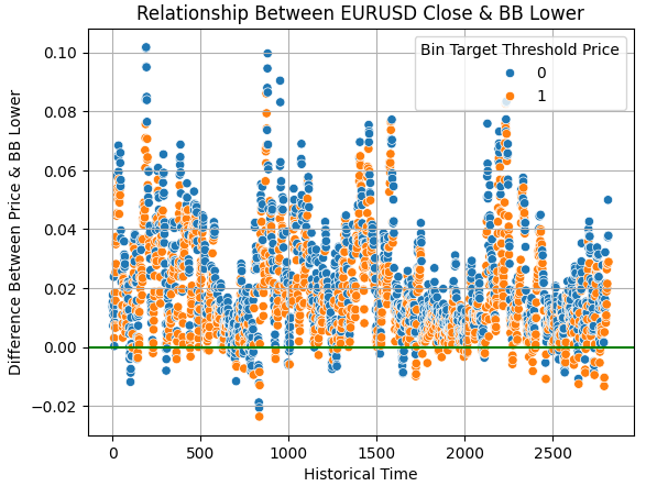
Figure 17: Both the upper and lower Bollinger Bands appear to set better decision boundaries than the RSI
Searching For High-Dimensional Trading Strategies With Unsupervised Machine Learning
At this point, we can begin to consider the possibility that market behavior is governed by more dimensions of variation than we can readily conceive. As humans, we struggle to reason beyond three dimensions, typically visualized along the X, Y, and Z axes. However, the market data used in this study spans eight dimensions: the open, high, low, close, upper, middle, and lower Bollinger Bands, as well as the RSI. This raises the possibility that a high-dimensional trading strategy exists—one that cannot be directly observed or intuitively understood.Unsupervised machine learning algorithms are well suited to detecting and exposing such high-dimensional structure in a form accessible to human interpretation. While many unsupervised techniques exist, our discussion focuses on a powerful nonlinear projection method known as Isometric Mapping (Isomap). These techniques are commonly referred to as manifold learning or dimensionality reduction algorithms. Their objective is to group similar observations closely while separating dissimilar observations as distinctly as possible.
A well-known dimensionality reduction method is Principal Component Analysis (PCA), which has been widely discussed in prior literature. However, PCA is a linear technique which may fail to capture complex nonlinear relationships present in market data. By contrast, Isomap—implemented via the sklearn.manifold library—may uncover nonlinear, high-dimensional relationships that could constitute a valid trading strategy beyond human intuition.
To begin, we load the Isomap library.
from sklearn.manifold import Isomap
Next, instantiate the encoder, and apply the fit_transform method to reduce our original eight-dimensional dataset to a two-dimensional representation.
enc = Isomap()

manifold = pd.DataFrame(enc.fit_transform(train.iloc[:,1:9]))

manifold
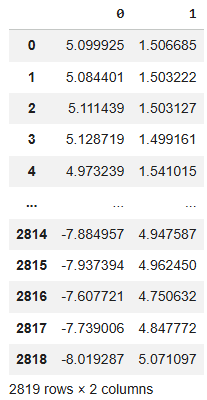
Figure 18: We employed isometric mapping to project all our market data down to just two columns
These learned manifolds are then appended to the original training set.
train['Iso 1'] = manifold.iloc[:,0]
train['Iso 2'] = manifold.iloc[:,1]
We next analyze the correlation between the learned manifold components and the original market variables. The first component exhibits positive correlation across all original price variables, implying that an increase in this component corresponds to rising open, high, low, and close prices. In contrast, the second component shows negative correlation, suggesting that a decline in this component is associated with rising price levels.
sns.heatmap(train.iloc[:,1:].corr())
plt.title('EURUSD Training Data Correlation Heatmap') 
Figure 19: The correlation matrix of our new training dataset
Using a scatter plot, we visualize the market data reduced from eight dimensions to two. While the resulting structure is not perfectly separated, meaningful patterns begin to emerge. Certain regions display well-defined bearish behavior, while others exhibit bullish characteristics. However, overlap remains, indicating residual noise that may affect downstream performance.
sns.scatterplot(data=train,x='Iso 1',y='Iso 2',hue='Bin Target Threshold Price')
plt.grid()
plt.title('Visualizing Our High Dimensional Data in 2 Dimensions') 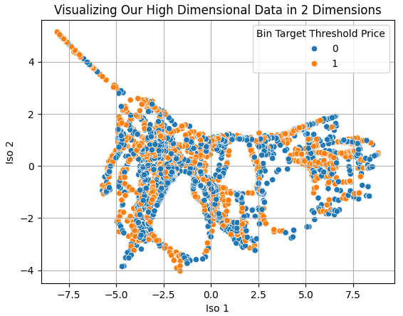
Figure 20: Dimensionality reduction algorithms allow us to visualize high dimensional data that would otherwise be impossible to fully visualize
Traditionally, learned manifold features are used to predict an original target variable. In our reimagining of this approach, we instead treat the learned manifold components as surrogate targets. The rationale is that these components may be more predictable than price itself. To test this hypothesis, we evaluate forecasting accuracy across several targets: price, the middle Bollinger Band, the RSI, and the two learned manifold components.
scores = []

from sklearn.ensemble import RandomForestClassifier

scores.append(np.mean(np.abs(cross_val_score(RandomForestClassifier(),train.iloc[:,1:9],train['Bin Target Threshold Price'],cv=tscv,scoring='accuracy'))))
scores.append(np.mean(np.abs(cross_val_score(RandomForestClassifier(),train.iloc[:,1:9],train['Bin Target Threshold BB Mid'],cv=tscv,scoring='accuracy'))))
scores.append(np.mean(np.abs(cross_val_score(RandomForestClassifier(),train.iloc[:,1:9],train['Bin Target Threshold RSI'],cv=tscv,scoring='accuracy'))))
scores.append(np.mean(np.abs(cross_val_score(RandomForestClassifier(),train.iloc[:,1:9],train['Bin Target 1'],cv=tscv,scoring='accuracy'))))
scores.append(np.mean(np.abs(cross_val_score(RandomForestClassifier(),train.iloc[:,1:9],train['Bin Target 2'],cv=tscv,scoring='accuracy'))))
Figure 21 presents the resulting bar plot. The accuracy achieved by directly predicting price is shown as a red dotted line. As expected, predicting the middle Bollinger Band yields significantly higher accuracy, as it represents a moving average and is inherently smoother than price. Notably, the second-best target is not the RSI, but rather the first Isomap component. This target exists in a high-dimensional space inaccessible to direct human reasoning, illustrating the power of dimensionality reduction techniques. However, as we have discussed in previous articles, improvements made in statistical metrics do not necessarily map to improved trading performance, a link to that discussion is provided here.
sns.barplot(scores)
plt.xticks([0,1,2,3,4],['Price','BB Mid','RSI','Iso 1','Iso 2'])
plt.axhline(scores[0],color='red',linestyle=':')
plt.ylabel('Cross Validation Accuracy 100%')
plt.xlabel('Candidate Target')
plt.title('Our Accuracy Predicting Different Targets Related to The EURUSD')
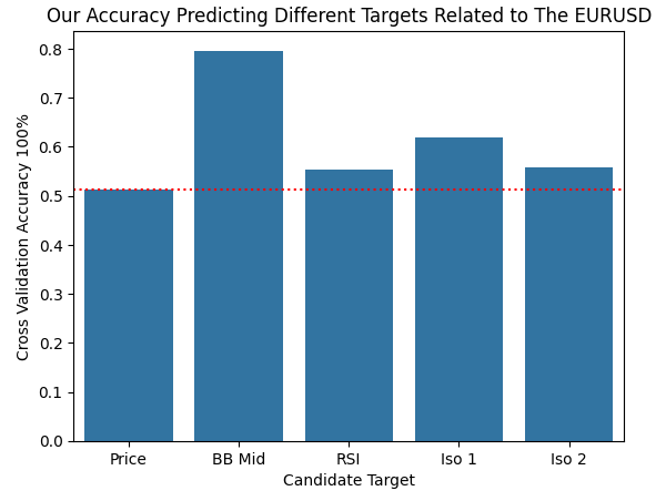
Figure 21: The second best target we could've modeled was embedded in dimensions too high for any form of human awareness
We then assess the material benefits of predicting this learned manifold instead of price. Following a familiar workflow, we fit a Random Forest regressor to forecast the first Isomap component and export the trained model to ONNX format. The model is deliberately named to reflect that it predicts the manifold produced by the Isomap algorithm.
initial_types = [('float_input',FloatTensorType([1,8]))]

final_types = [('float_output',FloatTensorType([1,1]))]

model = RandomForestRegressor()

model.fit(train.iloc[:,1:9],train['Bin Target 1'])

onnx_proto = convert_sklearn(model,initial_types=initial_types,final_types=final_types,target_opset=12)

onnx.save(onnx_proto,"EURUSD D1 Iso 1 RandomForestRegressor.onnx")
Final Attempts At Improvements
With these changes implemented, we test the revised application. We begin by loading the newly exported Random Forest model.//+------------------------------------------------------------------+ //| System resources | //+------------------------------------------------------------------+ #resource "\\Files\\EURUSD D1 Iso 1 RandomForestRegressor.onnx" as const uchar onnx_buffer[];
Then we must specify the model's inputs and outputs. Remember that unlike the previous iteration that employed 4 outputs, this model has a single output.
#define ONNX_INPUTS   8
#define ONNX_OUTPUTS  1
Trading rules are adjusted accordingly: when the forecast exceeds 0.5, we enter long positions; when it falls below 0.5, we enter short positions.
//+------------------------------------------------------------------+
//| Expert tick function                                             |
//+------------------------------------------------------------------+
void OnTick()
  {

//--- Check if a new candle has formed
   if(time_stamp != time_current)
     {

      //--- Prepare our ONNX model inputs
      vectorf onnx_inputs = {(float)iOpen(SYMBOL,TF_MAIN,SHIFT),
                             (float)iHigh(SYMBOL,TF_MAIN,SHIFT),
                             (float)iLow(SYMBOL,TF_MAIN,SHIFT),
                             (float)iClose(SYMBOL,TF_MAIN,SHIFT),
                             (float)bb_upper[0],
                             (float)bb_mid[0],
                             (float)bb_lower[0],
                             (float)rsi[0]};

      //--- Scale the model inputs appropriately
      for(int i = 0; i < ONNX_INPUTS;i++)
         {
            onnx_inputs[i] = ((onnx_inputs[i]-Z1[i])/Z2[i]);
         }

      //--- Obtain a forecast from our ONNX model
      OnnxRun(onnx_model,ONNX_DATA_TYPE_FLOAT,onnx_inputs,onnx_outputs);
      Comment("EURUSD Model Forecast: ",onnx_outputs);

      //--- Update current price levels
      double close = iClose(SYMBOL,TF_MAIN,SHIFT);

      //--- If we have no open positions
      if(PositionsTotal() == 0)
        {
         //--- Check for our trading signal
         if(onnx_outputs[0] < 0.5)
           {
            Trade.Sell(TradeHelper.MinVolume(),TradeHelper.GetSymbol(),TradeHelper.GetBid(),TradeHelper.GetBid() + (atr[0] * ATR_MULTIPLE),TradeHelper.GetBid() - (atr[0] * ATR_MULTIPLE),"");
           }

         else
            if(onnx_outputs[0] > 0.5)
              {
               Trade.Buy(TradeHelper.MinVolume(),TradeHelper.GetSymbol(),TradeHelper.GetAsk(),TradeHelper.GetAsk() - (atr[0] * ATR_MULTIPLE),TradeHelper.GetAsk() + (atr[0] * ATR_MULTIPLE),"");
              }
        }
     }
  }
//+------------------------------------------------------------------+
The resulting equity curve fails to meet expectations. While sporadic spikes in profitability are observed, the overall trend remains unstable and largely stationary around the starting balance. Despite this, the presence of unrealized equity spikes suggests that latent signal remains embedded within the high-dimensional structure.

Figure 22: The equity curve produced by our fifth iteration of our trading application reveals weaknesses in our high-dimensional trading strategy
Finally, examining the detailed performance statistics reveals mixed outcomes. The total number of trades increased substantially to 83, compared to the initial 14. However, net profitability deteriorated, and the proportion of profitable trades declined to 48%. Encouragingly, long trades were predominantly profitable. With further iteration and refined analysis, these results suggest there remains meaningful potential to uncover high-dimensional trading strategies that would otherwise remain undiscovered.

Figure 23: A detailed analysis of our final version of our trading application reveals the presence of unacceptable levels of noise
Conclusion
In conclusion, this article demonstrates how classical trading strategies can be rejuvenated with modern statistical algorithms to attain new levels of performance. Algorithmic trading is not a formulaic process; our success depends on persistence, reasoning, creativity, and energetic iteration. Moreover, the reader also walks away learning that, given the constantly growing availability of rich datasets from the MetaTrader 5 terminal, some trading strategies may remain concealed from human awareness, embedded in dimensions too high for direct observation.
By reimagining the application of unsupervised statistical algorithms, this article presents a numerically sound methodology for identifying high-dimensional trading strategies within your copy of the MetaTrader 5 terminal. Modern computers are capable of detecting complex high-dimensional structure in historical financial data, thereby discovering and learning trading strategies beyond human conception. This is truly exciting information to share and warrants more research. Ultimately, this article shows that the greatest benefit of algorithmic trading may lie in its capacity to reveal what is likely true—and what is likely not true—about financial markets we believed we already understood.
| File Name | File Description |
|---|---|
| Version_1.mq5 | The initial rule-based attempt we made to combine the Bollinger Bands and the Relative Strength Indicator. This application produced high probability trading signals, but the signals were obtained at low frequencies. |
| Version_2.mq5 | Our second iteration of the initial strategy employed more handwritten rules, but produced undesirable performance levels and reduced the signal in our trading strategy dramatically. |
| Version_3.mq5 | The third iteration of our Expert Advisor failed to employ statistical models to pick up appropriate trading signals. |
| Version_4.mq5 | The most profitable version of the trading application we managed to produce in our exercise. |
| Version_5.mq5 | The final iteration of our application attempted to learn high-dimensional trading strategies from the historical data, but failed to do so profitably. |
| Fetch_Data_Bollinger_Bands_RSI_Strategy.mq5 | The Jupyter Notebook we used to analyze our market data. |
| Bollinger_Band_RSI_Strategy.ipynb | The MQL5 script we used to write out historical market data to CSV for further analysis in Python. |
Warning: All rights to these materials are reserved by MetaQuotes Ltd. Copying or reprinting of these materials in whole or in part is prohibited.
This article was written by a user of the site and reflects their personal views. MetaQuotes Ltd is not responsible for the accuracy of the information presented, nor for any consequences resulting from the use of the solutions, strategies or recommendations described.

- Free trading apps
- Over 8,000 signals for copying
- Economic news for exploring financial markets
You agree to website policy and terms of use