ARIMA Forecasting Indicator in MQL5

Meteorologists do not read tea leaves when they make weather forecasts. They analyze what happened in the past to understand what will happen tomorrow. ARIMA model works in much the same way, but instead of clouds and pressure, it studies prices in financial markets.

ARIMA stands for “Autoregressive Integrated Moving Average” Model. It sounds scary, but in reality it is a rather logical system. Imagine you are trying to predict how much the EUR/USD pair will cost tomorrow based on how it has performed over the past few days.

Three pillars of the ARIMA model

Autoregression (AR) - memory of the past

The first part of the model is called autoregression. This beautiful word means a simple thing: today's price depends on yesterday's, the day before yesterday's, and so on. It's as if the market remembers its past and builds the future on its basis.

If EUR/USD has risen for three days in a row, there is a chance that it will rise tomorrow too. Not necessarily, but the trend may continue. The autoregressive part of the model captures these patterns by analyzing how much past values influence the current ones.

Math in simple words: imagine that you have the EUR/USD exchange rate for the last five days: 1.0800, 1.0825, 1.0850, 1.0875, 1.0900. Autoregression says: "Look, every day the exchange rate increased by about 25 points (0.0025), which means that tomorrow it will be around 1.0925." The model finds coefficients — numbers that show how strongly yesterday's price affects today's, the day before yesterday's on today's, and so on.

The formula looks something like this: tomorrow’s_price = 0.7 × today’s_price + 0.2 × yesterday’s_price + 0.1 × the day before yesterday’s_price. These coefficients 0.7, 0.2, 0.1 are selected by the model itself, analyzing the history. The higher the coefficient, the stronger the impact of this day on the forecast.

Integration (I) — taming chaos

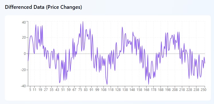
Imagine that you are looking at the EUR/USD chart and see a complete mess: 1.0800, 1.0850, 1.0820, 1.0880, 1.0860. The price jumps back and forth like a drunken sailor - no logic at first glance. It is such data that mathematicians call non—stationary, and traders call it a headache.

But here's the trick: instead of trying to make sense of the prices, ARIMA makes a smart move. It looks not at how much a currency pair is worth, but at how much it has changed for a day. Take the same numbers and count the differences: +50 points, -30 points, +60 points, -20 points. And suddenly, chaos turns into a pattern! The market swings between a rise of 50-60 points and a fall of 20-30 points.

It's as if you are not watching where the pendulum is, but only which way and with what force it is swinging. Mathematically, everything is simple: we take today's price, subtract yesterday's price, and get the change. Sometimes you should go further and take the "change of changes" — that is, second-order differentiation. It sounds scary, but the principle remains the same: looking for patterns where there are none at first glance.

Moving Average (MA) — learning from mistakes

And now the most interesting thing - the model can learn from its own mistakes. It sounds like science fiction, but the logic is ironclad. When ARIMA predicted EUR/USD at 1.0800 yesterday, and it was actually trading at 1.0825, this 25-point error was not just an annoying inaccuracy. This is information!

Imagine a friend who is always exactly 10 minutes late. When he says, "I'll be there at six," you already know it's really going to be at 6:10. The model does the same with its mistakes. If it predicts a price 10 points lower than the real one for three days in a row, it remembers these mistakes and the next time mentally adds: "I usually underestimate by 10 points, which means that the forecast needs to be adjusted."

The formula might look something like this: "Correction = 0.5 × yesterday's mistake + 0.3 × the day before yesterday's mistake." The model doesn't just make mistakes, it makes mistakes wisely, taking advantage of every mistake.

How ARIMA uses market psychology

Inertia of motion

Markets have inertia. If EUR/USD rises for several days in a row, everyone wants to buy it, which pushes the price even higher. ARIMA captures precisely this inertia.

In practice: the rate grows for five days from 1.0800 to 1.0900 (+20 points daily). The model places a lot of weight on recent days and predicts a continuation of the trend.

Return to the mean

At the same time, markets are striving for a "fair" level. If the price has deviated strongly in one direction, sooner or later it tries to come back.

An example: EUR/USD is usually trading in the range of 1.0800-1.0900. If it jumped to 1.1000 due to the news, the model will take into account through the moving average component that such extreme movements are usually adjusted.

Cyclical patterns

Many currency pairs exhibit cyclical behavior — weekly, monthly, or seasonal patterns. ARIMA can pick them up if set up correctly.

Disadvantages of the model: when ARIMA does not work

ARIMA is not the magic Grail. It operates with the assumption that the future is similar to the past. When this assumption is violated, the model makes inaccurate predictions.

The model does not do a good job when:

• Unexpected economic news is published
• The monetary policy of central banks is changing
• Geopolitical crises are taking place
• The market enters a new mode (for example, it moves from trend to flat)

ARIMA performs best in:

• Stable market conditions
• Periods without strong fundamental changes
• On instruments with pronounced technical patterns

Practical implementation in MQL5

Implementing a working ARIMA indicator is more than just formulas. We need a sophisticated architecture that can handle real-time data processing.

A module that evaluates the coefficients of the model is at the heart of the indicator. It uses the maximum likelihood method. This sounds complicated, but it's just a way to find the parameters at which the model best explains the observed data.

The data structure of the indicator includes several interconnected buffers: the main buffer of forecast values ForecastBuffer, the auxiliary buffer of historical prices PriceBuffer and the error buffer ErrorBuffer for storing the model residuals. This arrangement ensures optimal memory usage and high computing speed.

Initialization of the system involves creation of dynamic arrays for storing initial price data, a differentiated series, coefficients of autoregression and a moving average, as well as a residuals array. Initial values of the coefficients are set at 0.1, which ensures stability of the optimization algorithm at the initial stage.

int OnInit()
{
   // Setting indicator buffers for visualizing results
   SetIndexBuffer(0, ForecastBuffer, INDICATOR_DATA);
   SetIndexBuffer(1, PriceBuffer, INDICATOR_CALCULATIONS);
   SetIndexBuffer(2, ErrorBuffer, INDICATOR_CALCULATIONS);
   
   // Setting time series mode for correct operation with historical data
   ArraySetAsSeries(ForecastBuffer, true);
   ArraySetAsSeries(PriceBuffer, true);
   ArraySetAsSeries(ErrorBuffer, true);
   
   // Configuring forecast display with corresponding time shift
   PlotIndexSetString(0, PLOT_LABEL, "ARIMA Forecast");
   PlotIndexSetInteger(0, PLOT_SHIFT, forecast_bars);
   
   // Initializing working arrays with predefined sizes
   ArrayResize(prices, lookback);
   ArrayResize(differenced, lookback);
   ArrayResize(ar_coeffs, p);
   ArrayResize(ma_coeffs, q);
   ArrayResize(errors, lookback);
   
   // Setting initial values of model coefficients
   for(int i = 0; i < p; i++) ar_coeffs[i] = 0.1;
   for(int i = 0; i < q; i++) ma_coeffs[i] = 0.1;
   
   return(INIT_SUCCEEDED);
}

Input parameters of the model

The indicator is configured through a system of input parameters, each of which plays a critical role in determining the model's behavior. The lookback parameter determines the amount of historical data used to train the model, the forecast_bars parameter specifies the forecast horizon, and the triple of parameters p, d, q determines the specification of ARIMA model.

//--- Input parameters of model configuration
input int lookback = 200;        // Lookback period for ARIMA
input int forecast_bars = 20;    // Number of forecast time intervals
input int p = 3;                 // Order of autoregressive component
input int d = 1;                 // Degree of differentiation of a time series
input int q = 2;                 // Order of moving average component
input double learning_rate = 0.01; // Learning rate coefficient
input int max_iterations = 100;   // Maximum number of optimization iterations

Methodology for estimating model parameters

The central element of the algorithm is the function for calculating the logarithmic likelihood function, which serves as a criterion for the quality of the model's fit to the observed data. The implementation of this function is based on the assumption of a normal distribution of model residuals, which allows the use of an analytical expression for the probability density.

Likelihood function and calculation of residuals

The algorithm for calculating the log-likelihood function is an iterative process in which, for each time moment, residuals of the model are calculated as the difference between the observed value and the model forecast. The autoregressive component is formed as a linear combination of the previous values of the differentiated series, while the moving average component uses previous values of the model errors.

double ComputeLogLikelihood(double &data[], double &ar[], double &ma[])
{
   double ll = 0.0;
   double residuals[];
   ArrayResize(residuals, lookback);
   ArrayInitialize(residuals, 0.0);
   
   // Iterative calculation of model residuals
   for(int i = p; i < lookback; i++)
   {
      double ar_part = 0.0;
      double ma_part = 0.0;
      
      // Forming autoregressive component
      for(int j = 0; j < p && i - j - 1 >= 0; j++)
         ar_part += ar[j] * data[i - j - 1];
      
      // Forming moving average component
      for(int j = 0; j < q && i - j - 1 >= 0; j++)
         ma_part += ma[j] * errors[i - j - 1];
      
      // Calculating residuals and updating the error array
      residuals[i] = data[i] - (ar_part + ma_part);
      errors[i] = residuals[i];
      
      // Accumulating log-likelihood function
      ll -= 0.5 * MathLog(2 * M_PI) + 0.5 * residuals[i] * residuals[i];
   }
   
   return ll;
}

Coefficient optimization procedure

The coefficient optimization procedure is implemented using the gradient descent method with an adaptive step size. The algorithm iteratively updates the coefficient values in the direction opposite to the gradient of the objective function, ensuring convergence to the local optimum of the likelihood function.

void OptimizeCoefficients(double &data[])
{
   double temp_ar[], temp_ma[];
   ArrayCopy(temp_ar, ar_coeffs);
   ArrayCopy(temp_ma, ma_coeffs);
   
   double best_ll = -DBL_MAX;
   double grad_ar[], grad_ma[];
   ArrayResize(grad_ar, p);
   ArrayResize(grad_ma, q);
   
   // Iterative optimization process
   for(int iter = 0; iter < max_iterations; iter++)
   {
      ArrayInitialize(grad_ar, 0.0);
      ArrayInitialize(grad_ma, 0.0);
      
      // Calculating gradients of likelihood function
      for(int i = p; i < lookback; i++)
      {
         double ar_part = 0.0, ma_part = 0.0;
         
         // Forming model components
         for(int j = 0; j < p && i - j - 1 >= 0; j++)
            ar_part += temp_ar[j] * data[i - j - 1];
         for(int j = 0; j < q && i - j - 1 >= 0; j++)
            ma_part += temp_ma[j] * errors[i - j - 1];
         
         double residual = data[i] - (ar_part + ma_part);
         
         // Accumulating gradients by AR coefficients
         for(int j = 0; j < p && i - j - 1 >= 0; j++)
            grad_ar[j] += -residual * data[i - j - 1];
            
         // Accumulating gradients by MA coefficients
         for(int j = 0; j < q && i - j - 1 >= 0; j++)
            grad_ma[j] += -residual * errors[i - j - 1];
      }
      
      // Updating coefficients according to the gradient descent rule
      for(int j = 0; j < p; j++)
         temp_ar[j] += learning_rate * grad_ar[j] / lookback;
      for(int j = 0; j < q; j++)
         temp_ma[j] += learning_rate * grad_ma[j] / lookback;
      
      // Evaluating quality of current approximation
      double current_ll = ComputeLogLikelihood(data, temp_ar, temp_ma);
      
      // Stopping criterion and updating the optimal solution
      if(current_ll > best_ll)
      {
         best_ll = current_ll;
         ArrayCopy(ar_coeffs, temp_ar);
         ArrayCopy(ma_coeffs, temp_ma);
      }
      else
      {
         break; // Premature stop in the absence of improvement
      }
   }
}

Special attention is paid to the calculation of partial derivatives of the likelihood function for each of the optimized parameters. Gradients for autoregression coefficients are calculated as the sum of the products of residuals by the corresponding lag values of the differentiated series. While the gradients for moving average coefficients are determined through the products of the residuals by the previous error values.

Algorithm of forecasting and reversal of differentiation

Forecast values are generated recursively, starting from the last observed value of the time series. At each step of forecasting, the autoregressive component is calculated as a linear combination of previous values of the differentiated series with the corresponding coefficients. The moving average component is formed in a similar way, through a weighted sum of the previous residuals of the model.

The basic calculation procedure

The central OnCalculate function is the core of the computational process, that integrates all the components of the algorithm into a single data processing thread. The function performs sequential handling of incoming market data, application of the differentiation procedure, optimization of model parameters and generation of forecast values.

int OnCalculate(const int rates_total,
                const int prev_calculated,
                const datetime &time[],
                const double &open[],
                const double &high[],
                const double &low[],
                const double &close[],
                const long &tick_volume[],
                const long &volume[],
                const int &spread[])
{
   ArraySetAsSeries(close, true);
   ArraySetAsSeries(time, true);
   
   // Checking sufficiency of historical data
   if(rates_total < lookback + forecast_bars) return(0);
   
   // Forming array of closing prices
   for(int i = 0; i < lookback; i++)
   {
      prices[i] = close[i];
      PriceBuffer[i] = close[i];
   }
   
   // Applying differentiation procedure
   for(int i = 0; i < lookback - d; i++)
   {
      if(d == 1)
         differenced[i] = prices[i] - prices[i + 1];
      else if(d == 2)
         differenced[i] = (prices[i] - prices[i + 1]) - (prices[i + 1] - prices[i + 2]);
      else
         differenced[i] = prices[i];
   }
   
   // Optimizing AR and MA coefficients
   ArrayInitialize(errors, 0.0);
   OptimizeCoefficients(differenced);
   
   // Generating ARIMA forecast
   double forecast[];
   ArrayResize(forecast, forecast_bars);
   double undiff[];
   ArrayResize(undiff, forecast_bars);
   
   // Initializing forecasting process
   forecast[0] = prices[0];
   undiff[0] = prices[0];
   
   // Iterative forecast generation
   for(int i = 1; i < forecast_bars; i++)
   {
      double ar_part = 0.0;
      double ma_part = 0.0;
      
      // Calculating autoregressive component
      for(int j = 0; j < p && i - j - 1 >= 0; j++)
         ar_part += ar_coeffs[j] * (j < lookback ? differenced[j] : forecast[i - j - 1]);
      
      // Calculating moving average component
      for(int j = 0; j < q && i - j - 1 >= 0; j++)
         ma_part += ma_coeffs[j] * errors[j];
      
      // Forming forecast value
      forecast[i] = ar_part + ma_part;
      
      // Procedure of reversal of differentiation
      if(d == 1)
         undiff[i] = undiff[i - 1] + forecast[i];
      else if(d == 2)
         undiff[i] = undiff[i - 1] + (undiff[i - 1] - (i >= 2 ? undiff[i - 2] : prices[1])) + forecast[i];
      else
         undiff[i] = forecast[i];
      
      // Updating error array for following iterations
      errors[i % lookback] = forecast[i] - (i < lookback ? differenced[i] : 0.0);
   }
   
   // Filling output buffer with forecast values
   for(int i = 0; i < forecast_bars; i++)
   {
      ForecastBuffer[i] = undiff[i];
   }
   
   // Extending historical data for continuous display
   for(int i = forecast_bars; i < lookback; i++)
   {
      ForecastBuffer[i] = prices[i - forecast_bars];
   }
   
   return(rates_total);
}

The reverse differentiation procedure is a critical milestone that ensures the correct restoration of the initial scale of the forecast values. For the case of the first order of differentiation, each forecast value is obtained by summing the previous undifferentiated value with the corresponding forecast of the first difference. When using second-order differentiation, a more complex recursive formula is used that takes into account the curvature of the time series.

Computational aspects and performance optimization

The performance of the algorithm is largely determined by the correct organization of the computing process and the optimal use of processor resources. The main OnCalculate function is structured in such a way as to minimize the amount of redundant calculations when new market data arrives.

The differentiation procedure is implemented subject to different transformation orders. For first-order differentiation, a simple difference between neighboring observations is calculated, while for the second order, a second-difference formula is used. It allows you not only to eliminate the trend, but also changes in the trend rate.

A critical aspect of the implementation is memory management and correct operation with variable-length arrays. Using the ArrayResize and ArraySetAsSeries functions ensures that the data structure adapts to changing model parameters and data organization features in MetaTrader 5.

Calibration of parameters and adaptation to market conditions

Successful application of the ARIMA model in real trading conditions requires careful calibration of parameters, subject to the specifics of a particular financial instrument and the time horizon of the analysis. The lookback parameter determines the depth of historical analysis and should be sufficient to ensure the statistical significance of estimates, but not so large as to include outdated information.

The choice of p, d, and q orders of the model is a compromise between the accuracy of the data description and computational complexity. Increasing the order of autoregression p allows for more complex time dependencies. However, overcomplicating the model can result in overfitting and reducing prediction quality based on new data.

The learning rate parameter learning_rate requires particularly careful tuning, since a too large value can lead to fluctuations in the optimization algorithm, while a too small value slows down convergence to the optimum.

Statistical validation and evaluation of forecast quality

An objective assessment of the indicator quality requires the use of a set of statistical criteria that allow quantifying the accuracy of forecasting. The most informative metrics include the average absolute error, root of the root mean square error, and coefficient of determination.

Forecasting quality metrics

The implementation of forecast quality assessment functions allows for a quantitative analysis of the model performance and a comparison of various ARIMA specifications. The average absolute error provides an intuitive measure of the deviation of forecasts from real values, expressed in units of measurement of the original time series.

// Function of calculating average absolute error
double CalculateMAE(double &actual[], double &predicted[], int size)
{
   double mae = 0.0;
   for(int i = 0; i < size; i++)
   {
      mae += MathAbs(actual[i] - predicted[i]);
   }
   return mae / size;
}

// Function of calculating the root of the root mean square error
double CalculateRMSE(double &actual[], double &predicted[], int size)
{
   double mse = 0.0;
   for(int i = 0; i < size; i++)
   {
      double error = actual[i] - predicted[i];
      mse += error * error;
   }
   return MathSqrt(mse / size);
}

// Determination coefficient calculation function
double CalculateR2(double &actual[], double &predicted[], int size)
{
   double actual_mean = 0.0;
   for(int i = 0; i < size; i++)
      actual_mean += actual[i];
   actual_mean /= size;
   
   double ss_tot = 0.0, ss_res = 0.0;
   for(int i = 0; i < size; i++)
   {
      ss_tot += (actual[i] - actual_mean) * (actual[i] - actual_mean);
      ss_res += (actual[i] - predicted[i]) * (actual[i] - predicted[i]);
   }
   
   return 1.0 - (ss_res / ss_tot);
}

Diagnostics of model residuals

The analysis of model residuals is a critical aspect of validation, which allows us to identify systematic deviations from the model assumptions. The Ljung-Box test for autocorrelation of residuals provides a check on the adequacy of model specification, while the Jarque-Bera test allows you to assess the normality of the distribution of residuals.

// Function for calculating autocorrelation function of the residuals
double CalculateAutocorrelation(double &residuals[], int lag, int size)
{
   double mean = 0.0;
   for(int i = 0; i < size; i++)
      mean += residuals[i];
   mean /= size;
   
   double numerator = 0.0, denominator = 0.0;
   
   for(int i = lag; i < size; i++)
   {
      numerator += (residuals[i] - mean) * (residuals[i - lag] - mean);
   }
   
   for(int i = 0; i < size; i++)
   {
      denominator += (residuals[i] - mean) * (residuals[i] - mean);
   }
   
   return numerator / denominator;
}

// Ljung-Box statistic for testing autocorrelation
double LjungBoxTest(double &residuals[], int max_lag, int size)
{
   double lb_stat = 0.0;
   
   for(int k = 1; k <= max_lag; k++)
   {
      double rho_k = CalculateAutocorrelation(residuals, k, size);
      lb_stat += (rho_k * rho_k) / (size - k);
   }
   
   return size * (size + 2) * lb_stat;
}

The cross-validation procedure allows us to evaluate robustness of the model to changes within the training sample. The sliding window method provides a more realistic assessment of forecast quality under conditions close to real trading, when a model is successively applied to new data without revising the parameters.

Analysis of model residuals provides important information about the suitability of model assumptions to the characteristics of real data. Tests for autocorrelation of residuals allow you to identify unaccounted for time dependencies, while tests for normality of distribution of residuals check the correctness of the statistical model used.

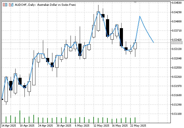
The indicator's output will be a forecast for the specified period:

Prospects for algorithm development and modification

Modern research in the field of financial time series analysis opens up wide opportunities for the development of the basic ARIMA model. Including seasonal components within the SARIMA model allows us to account for cyclical patterns which are characteristic for many financial instruments. Regularization methods such as L1 and L2 penalization can improve the model's robustness to outliers and prevent overfitting.

Adaptive algorithm modifications involving dynamic changes in model parameters depending on current market conditions are of particular interest for high-frequency trading. The integration of machine learning methods can provide automatic selection of the optimal model specification without involving an analyst.

Multidimensional extensions of the ARIMA model open up opportunities for simultaneous modeling of several interrelated financial instruments. This is especially important for portfolio management and arbitrage strategies.

Final considerations

The presented implementation of the ARIMA indicator in the MQL5 environment demonstrates the possibility of successful adaptation of classical econometric methods to the tasks of algorithmic trading. Strict adherence to statistical methodology combined with effective software implementation ensures the creation of a reliable tool for analyzing financial time series.

The practical application of the indicator requires a deep understanding of both mathematical foundations of a model and the specifics of the market in which it is used. The model performs obviously worse on systems with unstable trends.