
Data Science and ML (Part 35): NumPy in MQL5 – The Art of Making Complex Algorithms with Less Code

Contents
- Introduction
- Why NumPy?
- Vectors and Matrices initialization
- Mathematical functions
- Statistical functions
- Random numbers generators
- - Uniform distribution
- - Normal distribution
- - Exponential distribution
- - Binomial distribution
- - Poisson distribution
- - Shuffle
- - Random choice
- Fast Fourier Transform (FFT)
- - Standard Fast Fourier Transforms
- Linear algebra
- Polynomials (power series)
- Commonly used NumPy methods
- Coding ML models from scratch
- Conclusion
Believe you can and you're halfway there
-- Theodore Roosevelt.
Introduction
No programming language is entirely self-sufficient for every possible task we can think of creating through code, Every programming language depends on well-crafted tools which happen to be libraries, frameworks and modules to help tackle certain issues and convert some ideas into reality.
MQL5 is no exception. Designed primarily for algorithmic trading, its early functionality was mostly limited to trading operations. Unlike its predecessor, MQL4—considered a weaker language—MQL5 is far more powerful and capable. However, building a fully functional trading robot requires more than simply calling functions to place buy and sell trades.
To navigate the complexities of the financial markets, traders often deploy sophisticated mathematical operations including machine learning and Artificial Intelligence (AI). This has created a growing demand for optimized codebases and specialized frameworks that can handle complex computations efficiently.

Why NumPy?
When it comes to dealing with complex computations in MQL5, we have plenty of good libraries provided by MetaQuotes such as those found in Fuzzy, Stat, and the mighty Alglib (found in MetaEditor under MQL5\Include\Math).
These libraries have many functions suitable for programming complex expert advisors with minimal effort, however, most of the functions in these libraries are not that flexible due to the excessive use of arrays and object pointers, not to mention that some do require mathematical knowledge for one to use them properly.
Since the introduction of Matrices and Vectors MQL5 language has become more versatile and flexible when it comes to data storage and computations, these arrays which are in the form of objects which are accompanied by many built-in mathematical functions that once required manual implementations.
Due to the flexibility of matrices and vectors, we can extend them to something bigger, making a collection of various mathematical functions similar to those present in NumPy (Numerical Python, A python library that offers a collection of high-level mathematical functions including support for multidimensional arrays, masked arrays, and matrices).
It is fair to say that most of the functions offered by matrices and vectors in MQL5 took inspiration from NumPy as it can be seen from the docs, the syntax is very similar.
MQL5 | Python |
|---|---|
vector::Zeros(3); vector::Full(10); | numpy.zeros(3) numpy.full(10) |
According to the documentation, this similar syntax was introduced to "make it easier to translate algorithms and codes from Python to MQL5 with minimum efforts. A lot of data processing tasks, mathematical equations, neural networks, and machine learning tasks can be solved using ready-made Python methods and libraries".
This is true but, the functions provided by matrices and vectors aren't enough. We are still missing out plenty of crucial functions that we often need to translate these algorithms and codes from Python into MQL5, in this article, we will implement some of the most useful functions and methods from NumPy in MQL5 using a very close syntax to make it much easier to translate algorithms from Python programming language.
To keep the syntax similar to that of Python, we will implement the names of the functions in small letters. Starting with methods for initializing vectors and matrices.
Vectors and Matrices Initialization
To work with vectors and matrices, we need to have the methods for initializing them by populating them with some values. Below are some of the functions for the task.
Method | Description |
|---|---|
template <typename T> vector CNumpy::full(uint size, T fill_value) { return vector::Full(size, fill_value); } template <typename T> matrix CNumpy::full(uint rows, uint cols, T fill_value) { return matrix::Full(rows, cols, fill_value); } | Construct a new vector/matrix of given size/rows and columns, filled with a value. |
vector CNumpy::ones(uint size) { return vector::Ones(size); } matrix CNumpy::ones(uint rows, uint cols) { return matrix::Ones(rows, cols); } | Construct a new vector of a given size/matrix of given rows and columns, filled with ones |
vector CNumpy::zeros(uint size) { return vector::Zeros(size); } matrix CNumpy::zeros(uint rows, uint cols) { return matrix::Zeros(rows, cols); } | Construct a vector of a given size/matrix of given rows and columns, filled with zeros |
matrix CNumpy::eye(const uint rows, const uint cols, const int ndiag=0) { return matrix::Eye(rows, cols, ndiag); } | Construct a matrix with ones on the diagonal and zeros elsewhere. |
matrix CNumpy::identity(uint rows) { return matrix::Identity(rows, rows); } | Construct a square matrix with ones on the main diagonal. |
Despite their simplicity, these methods are crucial in creating placeholder matrices and vectors which are often used in transformations, padding, and augmentations.
Example usage:
#include <MALE5\Numpy\Numpy.mqh>
CNumpy np;
//+------------------------------------------------------------------+
//| Script program start function                                    |
//+------------------------------------------------------------------+
void OnStart()
  {
//--- Initialization

    // Vectors One-dimensional

    Print("numpy.full: ",np.full(10, 2));
    Print("numpy.ones: ",np.ones(10));
    Print("numpy.zeros: ",np.zeros(10));

    // Matrices Two-Dimensional

    Print("numpy.full:\n",np.full(3,3, 2));
    Print("numpy.ones:\n",np.ones(3,3));
    Print("numpy.zeros:\n",np.zeros(3,3));
    Print("numpy.eye:\n",np.eye(3,3));
    Print("numpy.identity:\n",np.identity(3));
 }
Mathematical Functions
This is a broad subject as there are a lot of mathematical functions to implement and describe for both vectors and matrices, and we'll discuss just some of them. Starting with mathematical constants.
Constants
Mathematical constants are as useful as the functions.
Constant | Description |
|---|---|
numpy.e | Euler’s constant, base of natural logarithms, Napier’s constant. |
numpy.euler_gamma | Defined as the limiting difference between the harmonic series and the natural logarithm. |
np.inf | IEEE 754 floating-point representation of (positive) infinity. |
np.nan |
|
| np.pi | Approximately equal to 3.14159, that is the ratio of a circle's circumference to its diameter. |
Example usage.
#include <MALE5\Numpy\Numpy.mqh>
CNumpy np;
//+------------------------------------------------------------------+
//| Script program start function                                    |
//+------------------------------------------------------------------+
void OnStart()
  {
//--- Mathematical functions

    Print("numpy.e: ",np.e);
    Print("numpy.euler_gamma: ",np.euler_gamma);
    Print("numpy.inf: ",np.inf);
    Print("numpy.nan: ",np.nan);
    Print("numpy.pi: ",np.pi);
 }
Functions
Below are some of the functions present in the CNumpy class.
| Method | Description |
|---|---|
vector CNumpy::add(const vector&a, const vector&b) { return a+b; }; matrix CNumpy::add(const matrix&a, const matrix&b) { return a+b; }; | Adds two vectors/matrices. |
vector CNumpy::subtract(const vector&a, const vector&b) { return a-b; }; matrix CNumpy::subtract(const matrix&a, const matrix&b) { return a-b; }; | Subtracts two vectors/matrices. |
vector CNumpy::multiply(const vector&a, const vector&b) { return a*b; }; matrix CNumpy::multiply(const matrix&a, const matrix&b) { return a*b; }; | Multiplies two vectors/matrices. |
vector CNumpy::divide(const vector&a, const vector&b) { return a/b; }; matrix CNumpy::divide(const matrix&a, const matrix&b) { return a/b; }; | Divides two vectors/matrices |
vector CNumpy::power(const vector&a, double n) { return MathPow(a, n); }; matrix CNumpy::power(const matrix&a, double n) { return MathPow(a, n); }; | It raises all elements in matrix/vector a to the power n. |
vector CNumpy::sqrt(const vector&a) { return MathSqrt(a); }; matrix CNumpy::sqrt(const matrix&a) { return MathSqrt(a); }; | Computes the square root of each element in the vector/matrix a. |
Example usage.
#include <MALE5\Numpy\Numpy.mqh>
CNumpy np;
//+------------------------------------------------------------------+
//| Script program start function                                    |
//+------------------------------------------------------------------+
void OnStart()
  {
//--- Mathematical functions

    vector a = {1,2,3,4,5};
    vector b = {1,2,3,4,5};

    Print("np.add: ",np.add(a, b));
    Print("np.subtract: ",np.subtract(a, b));
    Print("np.multiply: ",np.multiply(a, b));
    Print("np.divide: ",np.divide(a, b));
    Print("np.power: ",np.power(a, 2));
    Print("np.sqrt: ",np.sqrt(a));
    Print("np.log: ",np.log(a));
    Print("np.log1p: ",np.log1p(a));
 }
Statistical Functions
These can also be classified as mathematical functions, but unlike the basic mathematical operations, these functions help in providing analytical metrics from the given data. In machine learning, they are used mostly in feature engineering and normalization.
The below table represents some of the functions implemented in the MQL5-Numpy class.
Method | Descriptions |
|---|---|
double sum(const vector& v) { return v.Sum(); } double sum(const matrix& m) { return m.Sum(); }; vector sum(const matrix& m, ENUM_MATRIX_AXIS axis=AXIS_VERT) { return m.Sum(axis); }; | Calculates the sum of the vector/matrix elements, which can also be performed for the given axis (axes). |
double mean(const vector& v) { return v.Mean(); } double mean(const matrix& m) { return m.Mean(); }; vector mean(const matrix& m, ENUM_MATRIX_AXIS axis=AXIS_VERT) { return m.Mean(axis); }; |
|
double var(const vector& v) { return v.Var(); } double var(const matrix& m) { return m.Var(); }; vector var(const matrix& m, ENUM_MATRIX_AXIS axis=AXIS_VERT) { return m.Var(axis); }; |
|
double std(const vector& v) { return v.Std(); } double std(const matrix& m) { return m.Std(); }; vector std(const matrix& m, ENUM_MATRIX_AXIS axis=AXIS_VERT) { return m.Std(axis); }; |
|
double median(const vector& v) { return v.Median(); } double median(const matrix& m) { return m.Median(); }; vector median(const matrix& m, ENUM_MATRIX_AXIS axis=AXIS_VERT) { return m.Median(axis); }; | Computes the median of the vector/matrix elements. |
double percentile(const vector &v, int value) { return v.Percentile(value); } double percentile(const matrix &m, int value) { return m.Percentile(value); } vector percentile(const matrix &m, int value, ENUM_MATRIX_AXIS axis=AXIS_VERT) { return m.Percentile(value, axis); } | These functions calculate the specified percentile of values of a vector/matrix elements or elements along the specified axis. |
double quantile(const vector &v, int quantile_) { return v.Quantile(quantile_); } double quantile(const matrix &m, int quantile_) { return m.Quantile(quantile_); } vector quantile(const matrix &m, int quantile_, ENUM_MATRIX_AXIS axis=AXIS_VERT) { return m.Quantile(quantile_, axis); } | They calculate the specified quantile of values of matrix/vector elements or elements along the specified axis. |
vector cumsum(const vector& v) { return v.CumSum(); }; vector cumsum(const matrix& m) { return m.CumSum(); }; matrix cumsum(const matrix& m, ENUM_MATRIX_AXIS axis=AXIS_VERT) { return m.CumSum(axis); }; | These functions computes the cumulative sum of matrix/vector elements, including those along the given axis. |
vector cumprod(const vector& v) { return v.CumProd(); } vector cumprod(const matrix& m) { return m.CumProd(); }; matrix cumprod(const matrix& m, ENUM_MATRIX_AXIS axis=AXIS_VERT) { return m.CumProd(axis); }; | They return the cumulative product of matrix/vector elements, including those along the given axis. |
double average(const vector &v, const vector &weights) { return v.Average(weights); } double average(const matrix &m, const matrix &weights) { return m.Average(weights); } vector average(const matrix &m, const matrix &weights, ENUM_MATRIX_AXIS axis=AXIS_VERT) { return m.Average(weights, axis); } |
|
ulong argmax(const vector& v) { return v.ArgMax(); } ulong argmax(const matrix& m) { return m.ArgMax(); } vector argmax(const matrix& m, ENUM_MATRIX_AXIS axis=AXIS_VERT) { return m.ArgMax(axis); }; | They return the index of the maximum value. |
ulong argmin(const vector& v) { return v.ArgMin(); } ulong argmin(const matrix& m) { return m.ArgMin(); } vector argmin(const matrix& m, ENUM_MATRIX_AXIS axis=AXIS_VERT) { return m.ArgMin(axis); }; | They return the index of the minimum value. |
double min(const vector& v) { return v.Min(); } double min(const matrix& m) { return m.Min(); } vector min(const matrix& m, ENUM_MATRIX_AXIS axis=AXIS_VERT) { return m.Min(axis); }; | They return the minimum value in a vector/matrix, Including those along the specified axis. |
double max(const vector& v) { return v.Max(); } double max(const matrix& m) { return m.Max(); } vector max(const matrix& m, ENUM_MATRIX_AXIS axis=AXIS_VERT) { return m.Max(axis); }; | They return the maximum value in a vector/matrix, including those along the specified axis. |
double prod(const vector &v, double initial=1.0) { return v.Prod(initial); } double prod(const matrix &m, double initial) { return m.Prod(initial); } vector prod(const matrix &m, double initial, ENUM_MATRIX_AXIS axis=AXIS_VERT) { return m.Prod(axis, initial); } | They return the product of the matrix/vector elements, which can also be performed for the given axis. |
double ptp(const vector &v) { return v.Ptp(); } double ptp(const matrix &m) { return m.Ptp(); } vector ptp(const matrix &m, ENUM_MATRIX_AXIS axis=AXIS_VERT) { return m.Ptp(axis); } | They return the range of values of a matrix/vector or of the given matrix axis, equivalent to Max() - Min(). Ptp - Peak to peak. |
These functions are driven by built-in statistical functions for vectors and matrices as can be seen in the docs, all I did was create a NumPy similar syntax and wrap these functions.
Below is an example of how to use these functions.
#include <MALE5\Numpy\Numpy.mqh>
CNumpy np;
//+------------------------------------------------------------------+
//| Script program start function                                    |
//+------------------------------------------------------------------+
void OnStart()
  {
//--- Statistical functions

     vector z = {1,2,3,4,5};

     Print("np.sum: ", np.sum(z));
     Print("np.mean: ", np.mean(z));
     Print("np.var: ", np.var(z));
     Print("np.std: ", np.std(z));
     Print("np.median: ", np.median(z));
     Print("np.percentile: ", np.percentile(z, 75));
     Print("np.quantile: ", np.quantile(z, 75));
     Print("np.argmax: ", np.argmax(z));
     Print("np.argmin: ", np.argmin(z));
     Print("np.max: ", np.max(z));
     Print("np.min: ", np.min(z));
     Print("np.cumsum: ", np.cumsum(z));
     Print("np.cumprod: ", np.cumprod(z));
     Print("np.prod: ", np.prod(z));

     vector weights = {0.2,0.1,0.5,0.2,0.01};
     Print("np.average: ", np.average(z, weights));
     Print("np.ptp: ", np.ptp(z));
}
Random Numbers Generators
NumPy has a plenty of handy submodules, one of them being the random submodule.
The numpy.random submodule provides various random number generation functions based on the PCG64 random number generator (from NumPy 1.17+). Most of these methods are based on mathematical principles from probabilitytheory and statistical distributions.
In machine learning, we often generate random numbers for many use cases; We generate random numbers as initial starting weights for neural networks and many models that use iterative gradient descent-based methods for training, sometimes we even generate the random features that follow statistical distribution to get sample testing data for our models.
It is very crucial that the random numbers we generate follow statistical distribution something we can't achieve by using the native/built-in random number generation functions in MQL5.
Firstly, here is how you can set the random seed for the CNumpy.random submodule.
np.random.seed(42); Uniform Distribution #
We generate random numbers from a uniform distribution between some low and high values.
Formula:
Where R is a random number from [0,1].
 template <typename T>
 vector uniform(T low, T high, uint size=1)
  {
    vector res = vector::Zeros(size);
    for (uint i=0; i<size; i++)
       res[i] = low + (high - low) * (rand() / double(RAND_MAX));  // Normalize rand()

    return res;
  }
Usage.
Inside the Numpy.mqh file, a separate structure was created with the name CRandom which is then called inside the CNumpy class, this enables us to call a structure within a class, giving us a Python-like syntax.
class CNumpy
  {
protected:

public:
                     CNumpy(void);
                    ~CNumpy(void);

                    CRandom random;
  }
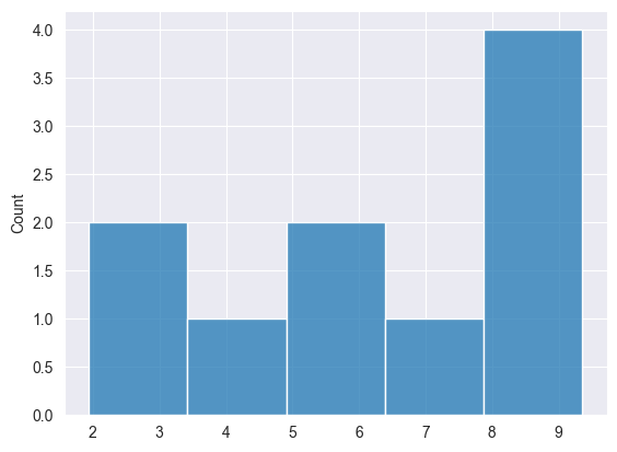
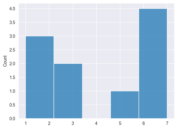
Print("np.random.uniform: ",np.random.uniform(1,10,10));
Outputs.
2025.03.16 15:03:15.102 Numpy np.random.uniform: [8.906552323984496,9.274605548265022,7.828760643330179,9.355082857753228,2.218420972319712,5.772331919309061,3.76067384868923,6.096438489944151,1.93908505508591,8.107272560808131]
We can visualize the results to see if the data is uniformly distributed.
Normal Distribution #
This method is used in many ML models, such as initializing neural network weights.
We can implement using Box-Muller transform.
Formula:
Where:
![]() are random numbers from [0,1]
are random numbers from [0,1]
 vector normal(uint size, double mean=0, double std=1)
   {
       vector results = {};  // Declare the results vector

       // We generate two random values in each iteration of the loop
       uint n = size / 2 + size % 2;  // If the size is odd, we need one extra iteration

       // Loop to generate pairs of normal numbers
       for (uint i = 0; i < n; i++)
       {
           // Generate two random uniform variables
           double u1 = MathRand() / 32768.0;  // Uniform [0,1] -> (MathRand() generates values from 0 to 32767)
           double u2 = MathRand() / 32768.0;  // Uniform [0,1]

           // Apply the Box-Muller transform to get two normal variables
           double z1 = MathSqrt(-2 * MathLog(u1)) * MathCos(2 * M_PI * u2);
           double z2 = MathSqrt(-2 * MathLog(u1)) * MathSin(2 * M_PI * u2);

           // Scale to the desired mean and standard deviation, and add them to the results
           results = push_back(results, mean + std * z1);
           if ((uint)results.Size() < size)  // Only add z2 if the size is not reached yet
               results = push_back(results, mean + std * z2);
       }

       // Return only the exact size of the results (if it's odd, we cut off one value)

       results.Resize(size);
       return results;
   }
Usage.
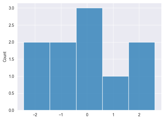
Print("np.random.normal: ",np.random.normal(10,0,1));
Outputs.
2025.03.16 15:33:08.791 Numpy test (US Tech 100,H1) np.random.normal: [-1.550635379340936,0.963285267506685,0.4587699653416977,-0.4813064556591148,-0.6919587880027229,1.649030932484221,-2.433415738330552,2.598464400400878,-0.2363726420659525,-0.1131299501178828]
Exponential Distribution #
The Exponential distribution is a probability distribution that describes the time between events in a Poisson process, where events occur continuously and independently at a constant average rate.
Given by the formula:
To generate exponentially distributed random numbers, we use the inverse transform sampling method. The formula is.
Where:
-
 is a uniform random number between 0 and 1.
 -
 is the rate parameter.
 vector  exponential(uint size, double lmbda=1.0)
   {
      vector res = vector::Zeros(size);
      for (uint i=0; i<size; i++)
         res[i] = -log((rand()/RAND_MAX)) / lmbda;

      return res;
   }
Usage.
Print("np.random.exponential: ",np.random.exponential(10));
Outputs.
2025.03.16 15:57:36.124 Numpy test (US Tech 100,H1) np.random.exponential: [0.4850272647406031,0.7617651806321184,1.09800210467871,2.658253432915927,0.5814831387699247,0.9920104404467721,0.7427922283035616,0.09323707153463576,0.2963563234048633,1.790326127008611]
Binomial Distribution #
This is a discrete probability distribution that models the number of successes in a fixed number of independent trials, each having the same probability of success.
Given by the formula.

We can implement it as follows.
// Function to generate a single Bernoulli(p) trial
int bernoulli(double p)
  {
    return (double)rand() / RAND_MAX < p ? 1 : 0;
  }
// Function to generate Binomial(n, p) samples
vector binomial(uint size, uint n, double p)
  {
    vector res = vector::Zeros(size);

    for (uint i = 0; i < size; i++)
      {
        int count = 0;
        for (uint j = 0; j < n; j++)
          count += bernoulli(p); // Sum of Bernoulli trials

        res[i] = count;
      }

    return res;
}
Usage.
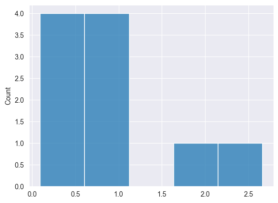
Print("np.random.binomial: ",np.random.binomial(10, 5, 0.5));
Outputs.
2025.03.16 19:35:20.346 Numpy test (US Tech 100,H1) np.random.binomial: [2,1,2,3,2,1,1,4,0,3]
Poisson Distribution #
This is a probability distribution that expresses the probability of a given number of events occurring in a fixed interval of time or space, given that these events happen at a constant average rate and independently of the time since the last event.
Formula.
Where:
-
 is the number of occurrences (0,1,2...)
 -
 (lambda) is the average rate of occurrences.
 - e is Euler's number.
int poisson(double lambda)
   {
       double L = exp(-lambda);
       double p = 1.0;
       int k = 0;

       while (p > L)
       {
           k++;
           p *= MathRand() / 32767.0; // Normalize MathRand() to (0,1)
       }

       return k - 1; // Since we increment k before checking the condition
   }
// We generate a vector of Poisson-distributed values
vector poisson(double lambda, int size)
{
    vector result = vector::Zeros(size);
    for (int i = 0; i < size; i++)
        result[i] = poisson(lambda);

    return result;
}
Usage.
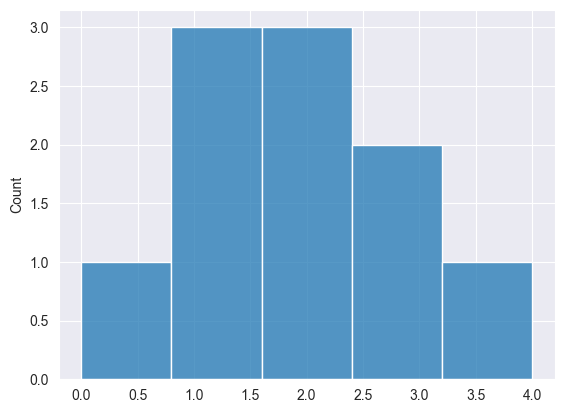
Print("np.random.poisson: ",np.random.poisson(4, 10));
Outputs.
2025.03.16 18:39:56.058 Numpy test (US Tech 100,H1) np.random.poisson: [6,6,5,1,3,1,1,3,6,7]
Shuffle #
When trying to train machine learning models to understand patterns in the data, we often shuffle the samples to help models understand the patterns present in the data and not the arrangement of the data.
The shuffle functionality is handy in such a situation.
Example usage.
vector data = {1,2,3,4,5,6,7,8,9,10};
np.random.shuffle(data);

Print("Shuffled: ",data);
Outputs.
2025.03.16 18:55:36.763 Numpy test (US Tech 100,H1) Shuffled: [6,4,9,2,3,10,1,7,8,5]
Random Choice #
Similarly to shuffle, this function samples the given 1-dimensional randomly but, with an option for shuffling with or without replacement.
template<typename T>
vector<T> choice(const vector<T> &v, uint size, bool replace=false)
With replacement.
Values will not be unique, the same items can be repeated in the resulting shuffled vector/array.
vector data = {1,2,3,4,5,6,7,8,9,10};

Print("np.random.choice replace=True: ",np.random.choice(data, (uint)data.Size(), true));
Outputs.
2025.03.16 19:11:53.520 Numpy test (US Tech 100,H1) np.random.choice replace=True: [5,3,9,2,1,3,4,7,8,3]
Without replacement.
The resulting shuffled vecor will have unique items just like they were in the original vector, only their order will be changed.
Print("np.random.choice replace=False: ",np.random.choice(data, (uint)data.Size(), false));
Outputs.
2025.03.16 19:11:53.520 Numpy test (US Tech 100,H1) np.random.choice replace=False: [8,4,3,10,5,7,1,9,6,2]
All functions in one place.
Example usage.
#include <MALE5\Numpy\Numpy.mqh>
CNumpy np;
//+------------------------------------------------------------------+
//| Script program start function                                    |
//+------------------------------------------------------------------+
void OnStart()
  {
//--- Random numbers generating

    np.random.seed(42);

    Print("---------------------------------------:");
    Print("np.random.uniform: ",np.random.uniform(1,10,10));
    Print("np.random.normal: ",np.random.normal(10,0,1));
    Print("np.random.exponential: ",np.random.exponential(10));
    Print("np.random.binomial: ",np.random.binomial(10, 5, 0.5));
    Print("np.random.poisson: ",np.random.poisson(4, 10));

    vector data = {1,2,3,4,5,6,7,8,9,10};
    //np.random.shuffle(data);
    //Print("Shuffled: ",data);

    Print("np.random.choice replace=True: ",np.random.choice(data, (uint)data.Size(), true));
    Print("np.random.choice replace=False: ",np.random.choice(data, (uint)data.Size(), false));
 }
Fast Fourier Transform (FFT) #
A fast Fourier transform (FFT) is an algorithm that computes the discrete Fourier transform (DFT) of a sequence, or its inverse (IDFT). A Fourier transform converts a signal from its original domain (often time or space) to a representation in the frequency domain and vice versa. The DFT is obtained by decomposing a sequence of values into components of different frequencies, read more.
This operation is useful in many fields such as.
- In signal and audio processing, it is used to convert time-domain sound waves to frequency spectra. In encoding the audio formats and filtering the noise.
- It is also used in image compression and in recognizing patterns from images.
- Data scientist often uses FFT to extract features from time series data.
The numpy.fft submodule is the one responsible for dealing with FFT.
In our CNumpy as it stands currently, I have implemented only the one-dimensional Standard FFT functions.
Before we explore the "Standard FFT" methods implemented in the class, let's understand the function for generating DFT frequencies.
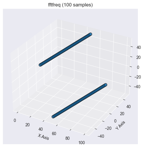
FFT frequency
When performing FFT on signal or data, the output is in the frequency domain, to interpret it, we need to know which frequency each element of the FFT corresponds to. This is where this method comes in.
This function returns the Discrete Fourier Transform (DFT) sample frequencies associated with an FFT of a given size. It helps determine the corresponding frequencies for each FFT coefficient.
vector fft_freq(int n, double d)
Example usage.
2025.03.17 11:11:10.165 Numpy test (US Tech 100,H1) np.fft.fftfreq: [0,0.1,0.2,0.3,0.4,-0.5,-0.4,-0.3,-0.2,-0.1]
Standard Fast Fourier Transforms #
FFT
This function computes the FFT of an input signal, converting it from the time domain to the frequency domain. It is an efficient algorithm to compute the Discrete Fourier Transform (DFT).
vector<complex> fft(const vector &x)
This function is built on top of CFastFourierTransform::FFTR1D a function provided by ALGLIB. Refer to ALGLIB for more information.
Example usage.
vector signal = {0. , 0.1, 0.2, 0.3, 0.4, 0.5, 0.6, 0.7, 0.8, 0.9};
Print("np.fft.fft: ",np.fft.fft(signal));
Output.
2025.03.17 11:28:16.739 Numpy test (US Tech 100,H1) np.fft.fft: [(4.5,0),(-0.4999999999999999,1.538841768587627),(-0.4999999999999999,0.6881909602355869),(-0.5000000000000002,0.3632712640026804),(-0.5000000000000002,0.1624598481164532),(-0.5,-3.061616997868383E-16),(-0.5000000000000002,-0.1624598481164532),(-0.5000000000000002,-0.3632712640026804),(-0.4999999999999999,-0.6881909602355869),(-0.4999999999999999,-1.538841768587627)]
Inverse FFT
This function computes the Inverse Fast Fourier Transform (IFFT), which converts frequency-domain data back to the time domain. It essentially undoes the effect of the previous method np.fft.fft.
vector ifft(const vectorc &fft_values)
Example usage.
vector signal = {0. , 0.1, 0.2, 0.3, 0.4, 0.5, 0.6, 0.7, 0.8, 0.9};

vectorc fft_res = np.fft.fft(signal); //perform fft
Print("np.fft.fft: ",fft_res); //fft results
Print("np.fft.ifft: ",np.fft.ifft(fft_res)); //Original signal
Outputs.
2025.03.17 11:45:04.537 Numpy test     np.fft.fft: [(4.5,0),(-0.4999999999999999,1.538841768587627),(-0.4999999999999999,0.6881909602355869),(-0.5000000000000002,0.3632712640026804),(-0.5000000000000002,0.1624598481164532),(-0.5,-3.061616997868383E-16),(-0.5000000000000002,-0.1624598481164532),(-0.5000000000000002,-0.3632712640026804),(-0.4999999999999999,-0.6881909602355869),(-0.4999999999999999,-1.538841768587627)]
2025.03.17 11:45:04.537 Numpy test     np.fft.ifft: [-4.440892098500626e-17,0.09999999999999991,0.1999999999999999,0.2999999999999999,0.4,0.5,0.6,0.7,0.8000000000000002,0.9]
Linear Algebra #
Linear algebra is a branch of mathematics that deals with vectors, matrices, and linear transformations. It is foundational to many fields such as physics, engineering, data science, etc.
NumPy provides the np.linalg module, a submodule dedicated to linear algebra functions. It offers almost all the functions for linear algebra such as for solving linear systems, computing eigenvalues/eigenvectors, and much more.
Below are some of the linear algebra functions implemented in the CNumpy class.
Method | Description |
|---|---|
matrix inv(const matrix &m) { return m.Inv(); } | Computes the multiplicative inverse of a square invertible matrix by the Jordan-Gauss method. |
double det(const matrix &m) { return m.Det(); } | Computes the determinant of a square invertible matrix. |
matrix kron(const matrix &a, const matrix &b) { return a.Kron(b); } matrix kron(const vector &a, const vector &b) { return a.Kron(b); } matrix kron(const vector &a, const matrix &b) { return a.Kron(b); } matrix kron(const matrix &a, const vector &b) { return a.Kron(b); } | They compute the Kronecker product of two matrices, matrix and vector, vector and matrix or two vectors. |
struct eigen_results_struct { vector eigenvalues; matrix eigenvectors; }; eigen_results_struct eig(const matrix &m) { eigen_results_struct res; if (!m.Eig(res.eigenvectors, res.eigenvalues)) printf("%s failed to calculate eigen vectors and values, error = %d",__FUNCTION__,GetLastError()); return res; } | This function computes the eigenvalues and right eigenvectors of a square matrix. |
double norm(const matrix &m, ENUM_MATRIX_NORM norm) { return m.Norm(norm); } double norm(const vector &v, ENUM_VECTOR_NORM norm) { return v.Norm(norm); } | Return matrix or vector norm, read more. |
svd_results_struct svd(const matrix &m) { svd_results_struct res; if (!m.SVD(res.U, res.V, res.singular_vectors)) printf("%s failed to calculate the SVD"); return res; } | Computes Singular Value Decomposition (SVD). |
vector solve(const matrix &a, const vector &b) { return a.Solve(b); } | Solve a linear matrix equation, or system of linear algebraic equations. |
vector lstsq(const matrix &a, const vector &b) { return a.LstSq(b); } | Calculates the least-squares solution of linear algebraic equations (for non-square or degenerate matrices). |
ulong matrix_rank(const matrix &m) { return m.Rank(); } | This function computes the rank of a matrix, which is the number of linearly independent rows or columns in the matrix. It is a key concept in understanding the solution space of a system of linear equations. |
matrix cholesky(const matrix &m) { vector values = eig(m).eigenvalues; for (ulong i=0; i<values.Size(); i++) { if (values[i]<=0) { printf("%s Failed Matrix is not positive definite",__FUNCTION__); return matrix::Zeros(0,0); } } matrix L; if (!m.Cholesky(L)) printf("%s Failed, Error = %d",__FUNCTION__, GetLastError()); return L; } | The Cholesky decomposition is used to factor a positive-definite matrix into the product of a lower triangular matrix and its transpose. |
matrix matrix_power(const matrix &m, uint exponent) { return m.Power(exponent); } | Computes the matrix raised to a specific integer power. More formally, it computes |
Example usage.
#include <MALE5\Numpy\Numpy.mqh>
CNumpy np;
//+------------------------------------------------------------------+
//| Script program start function                                    |
//+------------------------------------------------------------------+
void OnStart()
  {
    //--- Linear algebra


    matrix m = {{1,1,10},
                {1,0.5,1},
                {1.5,1,0.78}};

    Print("np.linalg.inv:\n",np.linalg.inv(m));
    Print("np.linalg.det: ",np.linalg.det(m));
    Print("np.linalg.det: ",np.linalg.kron(m, m));
    Print("np.linalg.eigenvalues:",np.linalg.eig(m).eigenvalues," eigenvectors: ",np.linalg.eig(m).eigenvectors);
    Print("np.linalg.norm: ",np.linalg.norm(m, MATRIX_NORM_P2));
    Print("np.linalg.svd u:\n",np.linalg.svd(m).U, "\nv:\n",np.linalg.svd(m).V);


    matrix a = {{1,1,10},
                {1,0.5,1},
                {1.5,1,0.78}};

    vector b = {1,2,3};

    Print("np.linalg.solve ",np.linalg.solve(a, b));
    Print("np.linalg.lstsq: ", np.linalg.lstsq(a, b));
    Print("np.linalg.matrix_rank: ", np.linalg.matrix_rank(a));
    Print("cholesky: ", np.linalg.cholesky(a));
    Print("matrix_power:\n", np.linalg.matrix_power(a, 2));
 }
Polynomials (Power Series) #
The numpy.polynomial submodule provides a set of powerful tools for creating, evaluating, differentiating, integrating, and manipulating polynomials. It is more numerically stable than using numpy.poly1d for polynomial operations.
There are different types of polynomials in the NumPy library in Python programming language but, in our CNumpy-MQL5 class, I have currently implemented a standard power base (Polynomial).
class CPolynomial: protected CNumpy
  {
protected:
   vector m_coeff;

   matrix vector21DMatrix(const vector &v)
    {
      matrix res = matrix::Zeros(v.Size(), 1);
      for (ulong r=0; r<v.Size(); r++)
         res[r][0] = v[r];

      return res;
    }

public:
                     CPolynomial(void);
                     CPolynomial(vector &coefficients); //for loading pre-trained model
                    ~CPolynomial(void);

                     vector fit(const vector &x, const vector &y, int degree);
  };
//+------------------------------------------------------------------+
//|                                                                  |
//+------------------------------------------------------------------+
CPolynomial::CPolynomial(void)
 {

 }
//+------------------------------------------------------------------+
//|                                                                  |
//+------------------------------------------------------------------+
CPolynomial::~CPolynomial(void)
 {

 }
//+------------------------------------------------------------------+
//|                                                                  |
//+------------------------------------------------------------------+
CPolynomial::CPolynomial(vector &coefficients):
m_coeff(coefficients)
 {

 }
//+------------------------------------------------------------------+
//|                                                                  |
//+------------------------------------------------------------------+
vector CPolynomial::fit(const vector &x, const vector &y, int degree)
 {
   //Constructing the vandermonde matrix
   matrix X = vander(x, degree+1, true);

   matrix temp1 =  X.Transpose().MatMul(X);
   matrix temp2 = X.Transpose().MatMul(vector21DMatrix(y));

   matrix coef_m = linalg.inv(temp1).MatMul(temp2);

   return (this.m_coeff = flatten(coef_m));
 }
Example usage.
#include <MALE5\Numpy\Numpy.mqh>
CNumpy np;
//+------------------------------------------------------------------+
//| Script program start function                                    |
//+------------------------------------------------------------------+
void OnStart()
  {
    //--- Polynomial

    vector X = {0. , 0.1, 0.2, 0.3, 0.4, 0.5, 0.6, 0.7, 0.8, 0.9};
    vector y = MathPow(X, 3) + 0.2 * np.random.randn(10);  // Cubic function with noise

    CPolynomial poly;

    Print("coef: ", poly.fit(X, y, 3));
 }
Outputs.
2025.03.17 14:01:43.026 Numpy test (US Tech 100,H1) coef: [-0.1905916844269999,2.3719065699851,-5.625684489899982,4.749058310806731]
Additionally, there are utility functions to help in polynomial manipulations, located in the main CNumpy class, these functions include.
Function | Description |
|---|---|
vector polyadd(const vector &p, const vector &q); | Adds two polynomials by aligning them based on their degree (length of coefficients). If one polynomial is shorter, it is padded with zeros before performing addition. |
vector polysub(const vector &p, const vector &q); | Subtracts two polynomials. |
vector polymul(const vector &p, const vector &q); | Multiplies two polynomials using distributive property, each term of p is multiplied by each term of q and the results are added. |
vector polyder(const vector &p, int m=1); | Computes the derivatives of the polynomial p, the derivative is computed by applying the standard rule for derivatives. Each term |
vector polyint(const vector &p, int m=1, double k=0.0) | Computes the integral of polynomial p, the integral of each term |
double polyval(const vector &p, double x); | Evaluates the polynomial at a specific value x by summing the terms of the polynomial, where each term is computes as |
struct polydiv_struct { vector quotient, remainder; }; polydiv_struct polydiv(const vector &p, const vector &q); | This function divides two polynomials and returns the quotient and remainder. |
Example usage.
#include <MALE5\Numpy\Numpy.mqh>
CNumpy np;
//+------------------------------------------------------------------+
//| Script program start function                                    |
//+------------------------------------------------------------------+
void OnStart()
  {
//--- Polynomial utils

    vector p = {1,-3, 2};
    vector q = {2,-4, 1};

    Print("polyadd: ",np.polyadd(p, q));
    Print("polysub: ",np.polysub(p, q));
    Print("polymul: ",np.polymul(p, q));
    Print("polyder:", np.polyder(p));
    Print("polyint:", np.polyint(p)); // Integral of polynomial
    Print("plyval x=2: ", np.polyval(p, 2)); // Evaluate polynomial at x = 2
    Print("polydiv:", np.polydiv(p, q).quotient," ",np.polydiv(p, q).remainder);
 }
Other commonly used NumPy methods
It is difficult to classify all the NumPy methods, below are has some of the most useful functions in the class that we haven't discussed yet.
Method | Description |
|---|---|
vector CNumpy::arange(uint stop) vector CNumpy::arange(int start, int stop, int step) | The first function creates a vector with a range of values at a specified interval. The second variant does the same thing but considers the step for incrementing the values. These two functions are useful for generating a vector of some number in ascending order. |
vector CNumpy::flatten(const matrix &m) vector CNumpy::ravel(const matrix &m) { return flatten(m); }; | They transform a 2D matrix into a 1D vector. We often end up with a matrix of maybe one row and one column that we need to converted into a vector for ease of use. |
matrix CNumpy::reshape(const vector &v,uint rows,uint cols) | Reshapes a 1D vector into a matrix of rows and columns (cols). |
matrix CNumpy::reshape(const matrix &m,uint rows,uint cols) | Reshapes a 2D matrix into a new shape (rows and cols). |
matrix CNumpy::expand_dims(const vector &v, uint axis) | Adds a new axis to the 1D vector, effectively converting it into a matrix. |
vector CNumpy::clip(const vector &v,double min,double max) | Clips values in a vector to be within a specified range (between min and max) values, useful for reducing extreme values and keeping the vector within a wanted range. |
vector CNumpy::argsort(const vector<T> &v) | Returns indices that would sort an array. |
vector CNumpy::sort(const vector<T> &v) | Sorts an array in ascending order. |
vector CNumpy::concat(const vector &v1, const vector &v2); vector CNumpy::concat(const vector &v1, const vector &v2, const vector &v3); | Concatenates more than one vector into one massive vector. |
matrix CNumpy::concat(const matrix &m1, const matrix &m2, ENUM_MATRIX_AXIS axis = AXIS_VERT) | When axis=0 concatenates the matrix along rows (stacks m1 with m2 matrices horizontally). When axis=1 concatenates the matrix along the columns (stacks m1 with m2 matrices vertically). |
matrix CNumpy::concat(const matrix &m, const vector &v, ENUM_MATRIX_AXIS axis = AXIS_VERT) | If axis = 0, appends the vector as a new row (only if its size matches the number of columns in the matrix). If axis = 1, appends the vector as a new column (only if its size matches the number of rows in the matrix). |
matrix CNumpy::dot(const matrix& a, const matrix& b); double CNumpy::dot(const vector& a, const vector& b); matrix CNumpy::dot(const matrix& a, const vector& b); | They compute the dot product (also known as the inner product) of two matrices, vectors, or a matrix and a vector. |
vector CNumpy::linspace(int start,int stop,uint num,bool endpoint=true) | It creates an array of evenly spaced numbers over a specified range (start, stop). num = the number of samples to generate. endpoint (default=true), stop is included, if set to false, stop is excluded. |
struct unique_struct { vector unique, count; }; unique_struct CNumpy::unique(const vector &v) | Returns the unique (unique) items in a vector and their counted number of appearances (count). |
Example usage.
#include <MALE5\Numpy\Numpy.mqh>
CNumpy np;
//+------------------------------------------------------------------+
//| Script program start function                                    |
//+------------------------------------------------------------------+
void OnStart()
  {
    //--- Common methods

    vector v = {1,2,3,4,5,6,7,8,9,10};

    Print("------------------------------------");
    Print("np.arange: ",np.arange(10));
    Print("np.arange: ",np.arange(1, 10, 2));

    matrix m = {
      {1,2,3,4,5},
      {6,7,8,9,10}
    };

    Print("np.flatten: ",np.flatten(m));
    Print("np.ravel: ",np.ravel(m));
    Print("np.reshape: ",np.reshape(v, 5, 2));
    Print("np.reshape: ",np.reshape(m, 2, 3));

    Print("np.expnad_dims: ",np.expand_dims(v, 1));
    Print("np.clip: ", np.clip(v, 3, 8));

    //--- Sorting

    Print("np.argsort: ",np.argsort(v));
    Print("np.sort: ",np.sort(v));

    //--- Others

    matrix z = {
      {1,2,3},
      {4,5,6},
      {7,8,9},
    };

    Print("np.concatenate: ",np.concat(v,  v));
    Print("np.concatenate:\n",np.concat(z,  z, AXIS_HORZ));

    vector y = {1,1,1};

    Print("np.concatenate:\n",np.concat(z,  y, AXIS_VERT));
    Print("np.dot: ",np.dot(v, v));
    Print("np.dot:\n",np.dot(z, z));
    Print("np.linspace: ",np.linspace(1, 10, 10, true));

    Print("np.unique: ",np.unique(v).unique, " count: ",np.unique(v).count);
 }
Outputs.
NJ      0       16:34:01.702    Numpy test (US Tech 100,H1)     ------------------------------------
PL      0       16:34:01.703    Numpy test (US Tech 100,H1)     np.arange: [0,1,2,3,4,5,6,7,8,9]
LG      0       16:34:01.703    Numpy test (US Tech 100,H1)     np.arange: [1,3,5,7,9]
QR      0       16:34:01.703    Numpy test (US Tech 100,H1)     np.flatten: [1,2,3,4,5,6,7,8,9,10]
QO      0       16:34:01.703    Numpy test (US Tech 100,H1)     np.ravel: [1,2,3,4,5,6,7,8,9,10]
EF      0       16:34:01.703    Numpy test (US Tech 100,H1)     np.reshape: [[1,2]
NL      0       16:34:01.703    Numpy test (US Tech 100,H1)      [3,4]
NK      0       16:34:01.703    Numpy test (US Tech 100,H1)      [5,6]
NQ      0       16:34:01.703    Numpy test (US Tech 100,H1)      [7,8]
HF      0       16:34:01.703    Numpy test (US Tech 100,H1)      [9,10]]
HD      0       16:34:01.703    Numpy test (US Tech 100,H1)     np.reshape: [[1,2,3]
QD      0       16:34:01.703    Numpy test (US Tech 100,H1)      [4,5,6]]
OH      0       16:34:01.703    Numpy test (US Tech 100,H1)     np.expnad_dims: [[1,2,3,4,5,6,7,8,9,10]]
PK      0       16:34:01.703    Numpy test (US Tech 100,H1)     np.clip: [3,3,3,4,5,6,7,8,8,8]
FM      0       16:34:01.703    Numpy test (US Tech 100,H1)     np.argsort: [0,1,2,3,4,5,6,7,8,9]
KD      0       16:34:01.703    Numpy test (US Tech 100,H1)     np.sort: [1,2,3,4,5,6,7,8,9,10]
FQ      0       16:34:01.703    Numpy test (US Tech 100,H1)     np.concatenate: [1,2,3,4,5,6,7,8,9,10,1,2,3,4,5,6,7,8,9,10]
FS      0       16:34:01.703    Numpy test (US Tech 100,H1)     np.concatenate:
PK      0       16:34:01.703    Numpy test (US Tech 100,H1)     [[1,2,3]
DM      0       16:34:01.703    Numpy test (US Tech 100,H1)      [4,5,6]
CJ      0       16:34:01.703    Numpy test (US Tech 100,H1)      [7,8,9]
IS      0       16:34:01.703    Numpy test (US Tech 100,H1)      [1,2,3]
DH      0       16:34:01.703    Numpy test (US Tech 100,H1)      [4,5,6]
PL      0       16:34:01.703    Numpy test (US Tech 100,H1)      [7,8,9]]
FQ      0       16:34:01.703    Numpy test (US Tech 100,H1)     np.concatenate:
CH      0       16:34:01.703    Numpy test (US Tech 100,H1)     [[1,2,3,1]
KN      0       16:34:01.703    Numpy test (US Tech 100,H1)      [4,5,6,1]
KH      0       16:34:01.703    Numpy test (US Tech 100,H1)      [7,8,9,1]]
JR      0       16:34:01.703    Numpy test (US Tech 100,H1)     np.dot: 385.0
PK      0       16:34:01.703    Numpy test (US Tech 100,H1)     np.dot:
JN      0       16:34:01.703    Numpy test (US Tech 100,H1)     [[30,36,42]
OH      0       16:34:01.703    Numpy test (US Tech 100,H1)      [66,81,96]
RN      0       16:34:01.703    Numpy test (US Tech 100,H1)      [102,126,150]]
RI      0       16:34:01.703    Numpy test (US Tech 100,H1)     np.linspace: [1,2,3,4,5,6,7,8,9,10]
MQ      0       16:34:01.703    Numpy test (US Tech 100,H1)     np.unique: [1,2,3,4,5,6,7,8,9,10] count: [1,1,1,1,1,1,1,1,1,1]
Coding Machine Learning Models from Scratch using MQL5-NumPy
As I explained earlier, the NumPy library is the backbone of many machine learning models you see implemented in Python programming language, due to the presence of a vast number of methods to help with arrays, matrices, basic mathematics, and even linear algebra. Now that we have a similar close in MQL5, let us attempt to use it to implement a simple machine learning model from scratch.
Using a Linear regression model as an example.
I found this code online, it's a linear regression model using gradient descent in its training function.
import numpy as np
from sklearn.metrics import mean_squared_error, r2_score

class LinearRegression:
    def __init__(self, learning_rate=0.01, epochs=1000):
        self.learning_rate = learning_rate
        self.epochs = epochs
        self.weights = None
        self.bias = None

    def fit(self, X, y):
        """
        Train the Linear Regression model using Gradient Descent.
        X: Input features (numpy array of shape [n_samples, n_features])
        y: Target values (numpy array of shape [n_samples,])
        """
        n_samples, n_features = X.shape
        self.weights = np.zeros(n_features)
        self.bias = 0

        for _ in range(self.epochs):
            y_pred = np.dot(X, self.weights) + self.bias  # Predictions

            # Compute Gradients
            dw = (1 / n_samples) * np.dot(X.T, (y_pred - y))
            db = (1 / n_samples) * np.sum(y_pred - y)

            # Update Parameters
            self.weights -= self.learning_rate * dw
            self.bias -= self.learning_rate * db

    def predict(self, X):
        """
        Predict output for the given input X.
        """
        return np.dot(X, self.weights) + self.bias

# Example Usage
if __name__ == "__main__":
    # Sample Data (X: Input features, y: Target values)
    X = np.array([[1], [2], [3], [4], [5]])  # Feature
    y = np.array([2, 4, 6, 8, 10])           # Target (y = 2x)

    # Create and Train Model
    model = LinearRegression(learning_rate=0.01, epochs=1000)
    model.fit(X, y)

    # Predictions
    y_pred = model.predict(X)

    # Evaluate Model
    print("Predictions:", y_pred)
    print("MSE:", mean_squared_error(y, y_pred))
    print("R² Score:", r2_score(y, y_pred))
Cell output.
Predictions: [2.06850809 4.04226297 6.01601785 7.98977273 9.96352761]
MSE: 0.0016341843485627612
R² Score: 0.9997957269564297
Pay attention to the fit function, we have a couple of NumPy methods in the training function. Since we also have these same functions in CNumpy let's do the same implementation in MQL5.
#include <MALE5\Numpy\Numpy.mqh>
//+------------------------------------------------------------------+
//| Script program start function                                    |
//+------------------------------------------------------------------+
void OnStart()
  {
//---
    // Sample Data (X: Input features, y: Target values)
    matrix X = {{1}, {2}, {3}, {4}, {5}};
    vector y = {2, 4, 6, 8, 10};

    // Create and Train Model
    CLinearRegression model(0.01, 1000);
    model.fit(X, y);

    // Predictions
    vector y_pred = model.predict(X);

    // Evaluate Model
    Print("Predictions: ", y_pred);
    Print("MSE: ", y_pred.RegressionMetric(y, REGRESSION_MSE));
    Print("R² Score: ", y_pred.RegressionMetric(y_pred, REGRESSION_R2));
  }
//+------------------------------------------------------------------+
//|                                                                  |
//+------------------------------------------------------------------+
class CLinearRegression
  {
protected:

   CNumpy np;
   double m_learning_rate;
   uint m_epochs;
   vector weights;
   double bias;

public:
                     CLinearRegression(double learning_rate=0.01, uint epochs=1000);
                    ~CLinearRegression(void);

                    void fit(const matrix &x, const vector &y);
                    vector predict(const matrix &X);
  };
//+------------------------------------------------------------------+
//|                                                                  |
//+------------------------------------------------------------------+
CLinearRegression::CLinearRegression(double learning_rate=0.01, uint epochs=1000):
 m_learning_rate(learning_rate),
 m_epochs(epochs)
 {

 }
//+------------------------------------------------------------------+
//|                                                                  |
//+------------------------------------------------------------------+
CLinearRegression::~CLinearRegression(void)
 {

 }
//+------------------------------------------------------------------+
//|                                                                  |
//+------------------------------------------------------------------+
void CLinearRegression::fit(const matrix &x, const vector &y)
 {
   ulong n_samples = x.Rows(), n_features = x.Cols();
   this.weights = np.zeros((uint)n_features);
   this.bias = 0.0;

//---

   for (uint i=0; i<m_epochs; i++)
      {
        matrix temp = np.dot(x, this.weights);
        vector y_pred = np.flatten(temp) + bias;

        // Compute Gradients

        temp = np.dot(x.Transpose(), (y_pred - y));

        vector dw = (1.0 / (double)n_samples) * np.flatten(temp);
        double db = (1.0 / (double)n_samples) * np.sum(y_pred - y);

        // Update Parameters

        this.weights -= this.m_learning_rate * dw;
        this.bias -= this.m_learning_rate * db;
      }

 }
//+------------------------------------------------------------------+
//|                                                                  |
//+------------------------------------------------------------------+
vector CLinearRegression::predict(const matrix &X)
 {
   matrix temp = np.dot(X, this.weights);

   return np.flatten(temp) + this.bias;
 }
Outputs.
RD      0       18:15:22.911    Linear regression from scratch (US Tech 100,H1) Predictions: [2.068508094061713,4.042262972785917,6.01601785151012,7.989772730234324,9.963527608958529]
KH      0       18:15:22.911    Linear regression from scratch (US Tech 100,H1) MSE: 0.0016341843485627612
RQ      0       18:15:22.911    Linear regression from scratch (US Tech 100,H1) R² Score: 1.0
Great, we got the same results from this model as we got in Python code.
Now What?
You have a powerful library and a collection of valuable methods that have been used to build countless machine learning and statistical algorithms in Python programming language, nothing stopping you from coding sophisticated trading robots equipped with complex calculations such as those you often see in Python.
As it stands currently the library still lacks most of the functions as it would take me months to write everything down so feel free to add one of your own, the functions present inside are the ones I use often or find myself wanting to use as I work with ML algorithms in MQL5.
The Python syntax in MQL5 can get confusing sometimes so don't hesitate to modify the function names to whatever is suitable for you.
Peace out.
Attachments Table
| Filename | Description |
|---|---|
| Include\Numpy.mqh | NumPy MQL5 clone, all the NumPy methods for MQL5 can be found in this file. |
| Scripts\Linear regression from scratch.mq5 | A script where the Linear regression example is implemented using CNumpy. |
| Scripts\Numpy test.mq5 | This script call all the methods from Numpy.mqh for testing purposes. Its a playground for all the methods discussed in this article. |
Warning: All rights to these materials are reserved by MetaQuotes Ltd. Copying or reprinting of these materials in whole or in part is prohibited.
This article was written by a user of the site and reflects their personal views. MetaQuotes Ltd is not responsible for the accuracy of the information presented, nor for any consequences resulting from the use of the solutions, strategies or recommendations described.

- Free trading apps
- Over 8,000 signals for copying
- Economic news for exploring financial markets
You agree to website policy and terms of use