
Neural Networks in Trading: Unified Trajectory Generation Model (UniTraj)

Introduction
The analysis of multi-agent behavior plays a crucial role in various domains, including finance, autonomous driving, and surveillance systems. Understanding agent actions requires solving several key tasks: object tracking, identification, trajectory modeling, and action recognition. Among these, trajectory modeling is particularly significant in the process of analyzing agent movements. Despite the complexities associated with environmental dynamics and subtle agent interactions, significant progress has recently been made in addressing this problem. The main achievements are concentrated in three key areas: trajectory prediction, missing data recovery, and spatiotemporal modeling.
However, most approaches remain specialized for specific tasks. This makes them difficult to generalize to other problems. Some tasks require both forward and backward spatiotemporal dependencies, which are often overlooked in prediction-oriented models. While some algorithms have successfully addressed the conditional calculation of multi-agent trajectories, they frequently fail to account for future trajectories. This limitation reduces their practical applicability in fully understanding movement, where predicting future trajectories is essential for planning subsequent actions rather than merely reconstructing past trajectories.
The paper "Deciphering Movement: Unified Trajectory Generation Model for Multi-Agent" presents the Unified TrajectoryGeneration (UniTraj) model, a universal framework integrating various trajectory-related tasks into a unified scheme. Specifically, the authors consolidate different types of input data into a single unified format: an arbitrary incomplete trajectory with a mask indicating the visibility of each agent at each time step. The model processes all task inputs uniformly as masked trajectories, aiming to generate complete trajectories based on incomplete ones.
To model spatiotemporal dependencies in different trajectory representations, the authors introduce the Ghost Spatial Masking (GSM) module, embedded within a Transformer-based encoder. Using the capabilities of recent popular state-space models (SSM), particularly the Mamba model, the authors adapt and enhance it into a bidirectional temporal encoder Mamba for long-term multi-agent trajectory generation. Additionally, they propose a simple yet effective Bidirectional Temporal Scaled (BTS) module, which comprehensively scans trajectories while preserving temporal relationships within the sequence. The experimental results presented in the paper confirm the robust and exceptional performance of the proposed method.
1. The UniTraj Algorithm
To handle various initial conditions within a single framework, the authors propose a unified generative trajectory model that treats any arbitrary input as a masked trajectory sequence. The visible regions of the trajectory serve as constraints or input data, while missing regions become targets for the generative task. This approach leads to the following problem definition:
It is necessary to determine the complete trajectory X[N, T, D], where N is number of agents, T represents the length of the trajectory, and D is the dimension of the agents' states. The state of agent i at time step t is denoted as xi,t[D]. Additionally, the algorithm uses a binary masking matrix M[N, T]. The variable mi,t equals 1 if the location of agent i is known at time t and 0 otherwise. Thus, the trajectory is divided into two segments by the mask: the visible region, defined as Xv=X⊙M, and the missing region, defined as Xm=X⊙(1−M). The objective is to create a complete trajectory Y'={X'v,X'm}, where X'v is a reconstructed trajectory and X'm is the newly generated trajectory. For consistency, the authors refer to the original trajectory as the ground truth Y=X={Xv, Xm}.
More formally, the goal is to train a generative model f(⋅) with parameters θ to output the complete trajectory Y'.
The general approach to estimating model parameters θ involves factorizing the joint trajectory distribution and maximizing the log-likelihood.
Consider agent i at time step t with position xi,t. First, the relative velocity 𝒗i,t, is computed by subtracting coordinates of adjacent time steps. For missing locations, values are filled with zero via element-wise multiplication with the mask. Additionally, a one-category vector 𝒄i,t is defined to represent agent categories. This categorization is crucial in sports scenarios where players may adopt specific offensive or defensive strategies. Agent features are projected into a high-dimensional feature vector 𝒇i,xt. The source feature vectors are calculated as follows:
![]()
where φx(⋅) is a projection function with weights 𝐖x, ⊙ represents element-wise multiplication, and ⊕ denotes concatenation.
The authors of the method implemented φx(⋅) using MLP. This approach incorporates information about position, velocity, visibility, and category to extract spatial features for subsequent analysis.
Unlike other sequential modeling tasks, it is crucial to account for dense social interactions. Existing studies on human interactions predominantly use attention mechanisms, such as cross-attention and graph-based attention, to capture this dynamic. However, since UniTraj addresses a unified task with arbitrary incomplete input data, the proposed model must explore spatiotemporal missing patterns. The authors introduce the Ghost Spatial Masking (GSM) module to abstract and generalize spatial structures of missing data. This module seamlessly integrates into the Transformer architecture without increasing model complexity.
Originally designed for modeling temporal dependencies in sequential data, the Transformer encoder in UniTraj applies a multi-head Self-Attention design in the spatial dimension. At each time step, the embedding of each of the N agents is processed as input to the Transformer encoder. This approach extracts order-invariant spatial features of agents, considering any possible agent ordering permutations in practical scenarios. Therefore, it is preferable to replace sinusoidal positional encoding with fully trainable encoding.
As a result, the Transformer encoder outputs spatial features Fs,xt for all agents at each time step t. These features are then concatenated along the temporal dimension to obtain spatial representations for the entire trajectory.
Given Mamba's capability to capture long-term temporal dependencies, the authors of UniTraj adapted it for integration into the proposed framework. However, adapting Mamba for unified trajectory generation is challenging due to the lack of a trajectory-specific architecture. Effective trajectory modeling requires capturing spatiotemporal features while handling missing data, which complicates the process.
To enhance temporal feature extraction while preserving missing relationships, a bidirectional temporal Mamba is introduced. This adaptation incorporates multiple residual Mamba blocks alongside an Bidirectional Temporal Scaled (BTS) module.
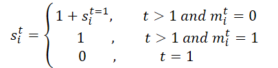
Initially, the mask M for the entire trajectory is processed. It is unfolded along the temporal dimension to generate M', facilitating the learning of temporal missing relationships by utilizing both original and reversed masks in the BTS module. This process generates a scaling matrix S and its inverse S'. Specifically, for agent i at time step t, si,t is computed as follows:
Subsequently, the scaling matrix S and its inverse S' are projected into the feature matrix:
![]()
where φs(⋅) represents projection functions with weights 𝐖s.
The authors implement φs(⋅) using MLP and the ReLU activation function. The proposed scaling matrix computes the distance from the last observation to the current time step, quantifying the impact of temporal gaps, especially when dealing with complex missing patterns. The key insight is that the influence of a variable diminishes over time when it has been missing for a certain period. Using a negative exponential function and ReLU ensures that the influence monotonically decays within a reasonable range between 0 and 1.
The encoding process aims to determine the parameters of a Gaussian distribution for the approximate posterior. Specifically, the mean μq and the standard deviation σq of the posterior Gaussian distribution are computed as follows:
![]()
We sample latent variables 𝒁 from the prior Gaussian distribution 𝒩(0, I).
To enhance the model's ability to generate plausible trajectories, we combine this function Fz,x with latent variable 𝒁 before feeding it into the decoder. The trajectory generation process is then computed as follows:
![]()
where φdec is the decoder function, implemented using an MLP.
In the presence of an arbitrary incomplete trajectory, the UniTraj model generates a complete trajectory. During the training process, the reconstruction error for visible areas and the restoration error for masked data are calculated.
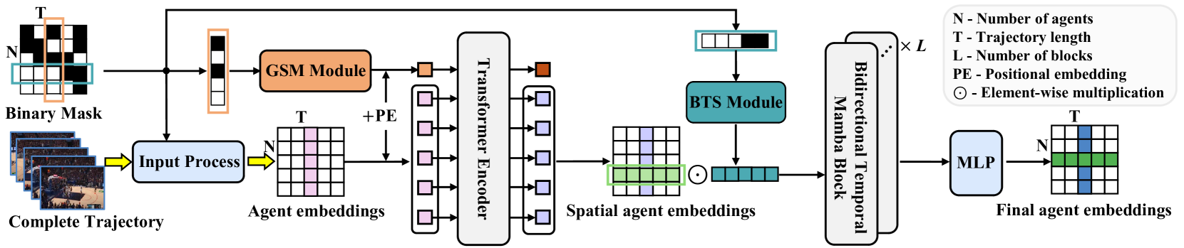
The author's visualization of the UniTraj method is presented below.
2. Implementation in MQL5
After considering the theoretical aspects of the UniTraj method, we move on to the practical part of our article, in which we implement our vision of the proposed approaches using MQL5. It is important to note that the proposed algorithm structurally differs from the methods we have previously examined.
The first notable difference is the masking process. When passing input data to the model, the authors suggest preparing an additional mask that determines which data the model can see and which it must generate. This adds an extra step to the workflow and increases decision-making time, which is undesirable. Therefore, we aim to incorporate mask generation within the model itself.
The second aspect is the transmission of the complete trajectory to the model. While obtaining a full trajectory is possible during testing, it is not available in real-world deployment. The model allows missing data to be masked and subsequently reconstructed, but we must still provide a larger tensor to the model. This leads to increased memory consumption and additional overhead for data transmission, ultimately affecting processing speed. A potential solution is to limit the transmission
to historical data only during both training and deployment. However, doing so would compromise a significant portion of the method's functionality.
To balance efficiency and accuracy, I have decided to divide the data transmission into two parts: historical data and the future trajectory. The latter is provided only during the training phase to extract spatial-temporal dependencies. During real-time execution, the future trajectory tensor is omitted, and the model operates in a predictive mode.
Additionally, this implementation required certain modifications on the OpenCL side.
2.1 Enhancements to the OpenCL Program
As the first step in our implementation, we prepare new kernel functions within the OpenCL program. The primary addition is the UniTrajPrepare kernel, responsible for data preprocessing. This kernel concatenates historical data with the known future trajectory while applying the appropriate masking.
The kernel parameters include pointers to 5 data buffers: 4 for input data and one for output results. It also requires parameters defining the depth of the historical data analysis and the planning horizon.
__kernel void UniTrajPrepare(__global const float *history,
                             __global const float *h_mask,
                             __global const float *future,
                             __global const float *f_mask,
                             __global float *output,
                             const int h_total,
                             const int f_total
                            )
  {
   const size_t i = get_global_id(0);
   const size_t v = get_global_id(1);
   const size_t variables = get_global_size(1);
We plan the execution of the kernel in a two-dimensional task space. The first dimension is the size of the larger of the two time periods (history depth and planning horizon). The second dimension will indicate the number of parameters analyzed.
In the kernel body, we first identify a thread in a given task space. We also determine the offset in the data buffers.
   const int shift_in = i * variables + v;
   const int shift_out = 3 * shift_in;
   const int shift_f_out = 3 * (h_total * variables + v);
Next we work with historical data. Here we first determine the rate of change of the parameter taking into account the mask. And then we save the parameter value in the results buffer taking into account the max, the previously calculated speed and the mask itself.
//--- history
   if(i < h_total)
     {
      float mask = h_mask[shift_in];
      float h = history[shift_in];
      float v = (i < (h_total - 1) && mask != 0 ? (history[shift_in + variables] - h) * mask : 0);
      if(isnan(v) || isinf(v))
         v = h = mask = 0;
      output[shift_out] = h * mask;
      output[shift_out + 1] = v;
      output[shift_out + 2] = mask;
     }
We calculate similar parameters for future values.
//--- future
   if(i < f_total)
     {
      float mask = f_mask[shift_in];
      float f = future[shift_in];
      float v = (i < (f_total - 1) && mask != 0 ? (future[shift_in + variables] - f) * mask : 0);
      if(isnan(v) || isinf(v))
         v = f = mask = 0;
      output[shift_f_out + shift_out] = f * mask;
      output[shift_f_out + shift_out + 1] = v;
      output[shift_f_out + shift_out + 2] = mask;
     }
  }
Next we save the kernel of the reverse pass of the above operations: UniTrajPrepareGrad.
__kernel void UniTrajPrepareGrad(__global float *history_gr,
                                 __global float *future_gr,
                                 __global const float *output,
                                 __global const float *output_gr,
                                 const int h_total,
                                 const int f_total
                                )
  {
   const size_t i = get_global_id(0);
   const size_t v = get_global_id(1);
   const size_t variables = get_global_size(1);
Note that we do not specify pointers to the source data and mask buffers in the parameters of the backward pass method. Instead, we use the result buffer of the UniTrajPrepare feed-forward kernel, which stores the specified data. Also, we do not pass the error gradient to the mask layer, as it does not make sense.
The task space of the backpropagation kernel is identical to that discussed above for the feed-forward kernel.
In the kernel body, we identify the current thread in the task space and determine the offset into the data buffers.
   const int shift_in = i * variables + v;
   const int shift_out = 3 * shift_in;
   const int shift_f_out = 3 * (h_total * variables + v);
Similar to the feed-forward kernel, we organize the work in 2 stages. First, we distribute the error gradient to the historical data level.
//--- history
   if(i < h_total)
     {
      float mask = output[shift_out + 2];
      float grad = 0;
      if(mask > 0)
        {
         grad = output_gr[shift_out] * mask;
         grad -= (i < (h_total - 1) && mask != 0 ? (output_gr[shift_out + 1]) * mask : 0);
         grad += (i > 0 ? output[shift_out + 1 - 3 * variables] * output[shift_out + 2 - 3 * variables] : 0);
         if(isnan(grad) || isinf(grad))
            grad = 0;
         //---
        }
      history_gr[shift_in] = grad;
     }
And then we propagate the error gradient to the known predicted values.
//--- future
   if(i < f_total)
     {
      float mask = output[shift_f_out + shift_out + 2];
      float grad = 0;
      if(mask > 0)
        {
         grad = output_gr[shift_f_out + shift_out] * mask;
         grad -= (i < (h_total - 1) && mask != 0 ? (output_gr[shift_f_out + shift_out + 1]) * mask : 0);
         grad += (i > 0 ? output[shift_f_out + shift_out + 1 - 3 * variables] *
                          output[shift_f_out + shift_out + 2 - 3 * variables] : 0);
         if(isnan(grad) || isinf(grad))
            grad = 0;
         //---
        }
      future_gr[shift_in] = grad;
     }
  }
Another algorithm that we need to implement on the OpenCL side is creating a scaling matrix. In the UniTrajBTS kernel, we calculate the direct and inverse scaling matrices.
Here we also use the feed-forward results of the data preparation kernel as input. Based on its data, we calculate the offset from the last unmasked value in the forward and backward directions, which we save in the corresponding data buffers.
__kernel void UniTrajBTS(__global const float * concat_inp,
                         __global float * d_forw,
                         __global float * d_bakw,
                         const int total
                        )
  {
   const size_t i = get_global_id(0);
   const size_t v = get_global_id(1);
   const size_t variables = get_global_size(1);
We use a two-dimensional task space. But in the first dimension, we will have only 2 threads, which correspond to the calculation of the direct and inverse scaling matrix. In the second dimension, as before, we will indicate the number of variables being analyzed.
After identifying the thread in the task space, we split the kernel algorithm depending on the value of the first dimension.
   if(i == 0)
     {
      const int step = variables * 3;
      const int start = v * 3 + 2;
      float last = 0;
      d_forw[v] = 0;
      for(int p = 1; p < total; p++)
        {
         float m = concat_inp[start + p * step];
         d_forw[p * variables + v] = last = 1 + (1 - m) * last;
        }
     }
When computing the direct scaling matrix, we determine the offset to the mask of the first element of the analyzed variable and the step to the next element. We then iterate sequentially through the masks of the analyzed element, calculating the scaling coefficients according to the given formula.
For the inverse scaling matrix, the algorithm remains identical. Except that we determine the offset to the last element and iterate in reverse order.
   else
     {
      const int step = -(variables * 3);
      const int start = (total - 1) * variables + v * 3 + 2;
      float last = 0;
      d_bakw[(total - 1) + v] = 0;
      for(int p = 1; p < total; p++)
        {
         float m = concat_inp[start + p * step];
         d_bakw[(total - 1 - p) * variables + v] = last = 1 + (1 - m) * last;
        }
     }
  }
Note that the presented algorithm works only with masks, for which the distribution of the error gradient does not make sense. For this reason, we do not create a backpropagation kernel for this algorithm. This concludes our operations on the OpenCL program side. You can find its full code in the attachment.
2.2 Implementing the UniTraj algorithm
After preparatory operations on the OpenCL program side, we move on to implementing the proposed approaches on the side of the main program. The UniTraj algorithm will be implemented within the CNeuronUniTraj class. Its structure is presented below.
class CNeuronUniTraj    :  public CNeuronBaseOCL
  {
protected:
   uint              iVariables;
   float             fDropout;
   //---
   CBufferFloat      cHistoryMask;
   CBufferFloat      cFutureMask;
   CNeuronBaseOCL    cData;
   CNeuronLearnabledPE cPE;
   CNeuronMVMHAttentionMLKV   cEncoder;
   CNeuronBaseOCL    cDForw;
   CNeuronBaseOCL    cDBakw;
   CNeuronConvOCL    cProjDForw;
   CNeuronConvOCL    cProjDBakw;
   CNeuronBaseOCL    cDataDForw;
   CNeuronBaseOCL    cDataDBakw;
   CNeuronBaseOCL    cConcatDataDForwBakw;
   CNeuronMambaBlockOCL cSSM[4];
   CNeuronConvOCL    cStat;
   CNeuronTransposeOCL cTranspStat;
   CVAE              cVAE;
   CNeuronTransposeOCL cTranspVAE;
   CNeuronConvOCL    cDecoder[2];
   CNeuronTransposeOCL cTranspResult;
   //---
   virtual bool      Prepare(const CBufferFloat* history, const CBufferFloat* future);
   virtual bool      PrepareGrad(CBufferFloat* history_gr, CBufferFloat* future_gr);
   virtual bool      BTS(void);
   //---
   virtual bool      feedForward(CNeuronBaseOCL *NeuronOCL) override { return feedForward(NeuronOCL, NULL); }
   virtual bool      feedForward(CNeuronBaseOCL *NeuronOCL, CBufferFloat *SecondInput) override;
   //---
   virtual bool      calcInputGradients(CNeuronBaseOCL *NeuronOCL) override
                                       { return calcInputGradients(NeuronOCL, NULL, NULL, None); }
   virtual bool      updateInputWeights(CNeuronBaseOCL *NeuronOCL) override
                                       { return updateInputWeights(NeuronOCL, NULL); }
   virtual bool      calcInputGradients(CNeuronBaseOCL *NeuronOCL, CBufferFloat *SecondInput,
                                                                   CBufferFloat *SecondGradient,
                                                            ENUM_ACTIVATION SecondActivation = None) override;
   virtual bool      updateInputWeights(CNeuronBaseOCL *NeuronOCL, CBufferFloat *second) override;
   //---

public:
                     CNeuronUniTraj(void) {};
                    ~CNeuronUniTraj(void) {};
   //---
   virtual bool      Init(uint numOutputs, uint myIndex, COpenCLMy *open_cl,
                          uint window, uint window_key, uint heads, uint units_count,
                          uint forecast, float dropout, ENUM_OPTIMIZATION optimization_type, uint batch);
   //---
   virtual int       Type(void)   const   {  return defNeuronUniTrajOCL; }
   //---
   virtual bool      Save(int const file_handle);
   virtual bool      Load(int const file_handle);
   //---
   virtual bool      WeightsUpdate(CNeuronBaseOCL *source, float tau);
   virtual void      SetOpenCL(COpenCLMy *obj);
  };
As you can see, the class structure declares a large number of internal objects, whose functionality we will explore step by step as we proceed with method implementation. All objects are declared statically. This allows us to leave the class constructor and destructor empty, while memory operations will be delegated to the system.
All internal objects are initialized in the Init method. In its parameters, we obtain the main constants that allow us to uniquely identify the architecture of the object.
bool CNeuronUniTraj::Init(uint numOutputs, uint myIndex, COpenCLMy *open_cl,
                          uint window, uint window_key, uint heads, uint units_count,
                          uint forecast, float dropout, ENUM_OPTIMIZATION optimization_type, uint batch)
  {
   if(!CNeuronBaseOCL::Init(numOutputs, myIndex, open_cl, window * (units_count + forecast),
                                                                   optimization_type, batch))
      return false;
Within the method body, following established convention, we first invoke the identically named method of the parent class, which already implements the essential initialization controls for inherited objects.
After the successful execution of the parent class operations, we store the constants received from the external program. These include the number of analyzed variables in the input data and the proportion of elements masked during the training process.
   iVariables = window;
   fDropout = MathMax(MathMin(dropout, 1), 0);
Next, we move on to initializing the declared objects. Here we first create buffers to mask historical and forecast data.
   if(!cHistoryMask.BufferInit(iVariables * units_count, 1) ||
      !cHistoryMask.BufferCreate(OpenCL))
      return false;
   if(!cFutureMask.BufferInit(iVariables * forecast, 1) ||
      !cFutureMask.BufferCreate(OpenCL))
      return false;
Then we initialize the inner layer of concatenated source data.
   if(!cData.Init(0, 0, OpenCL, 3 * iVariables * (units_count + forecast), optimization, iBatch))
      return false;
And create a similarly sized learnable positional coding layer.
   if(!cPE.Init(0, 1, OpenCL, cData.Neurons(), optimization, iBatch))
      return false;
This is followed by the Transformer encoder which is used to extract spatial-temporal dependencies.
   if(!cEncoder.Init(0, 2, OpenCL, 3, window_key, heads, (heads + 1) / 2, iVariables, 1, 1,
                                                  (units_count + forecast), optimization, iBatch))
      return false;
It is worth noting that the authors conducted a series of experiments and concluded that the optimal performance of the method is achieved when using a single Transformer Encoder block and four Mamba blocks. Therefore, in this case, we utilize only one Encoder layer.
Additionally, note that the input window size is set to "3", corresponding to three parameters of a single indicator at each time step (value, velocity, and mask). The sequence length is determined by the number of analyzed variables, while the number of independent channels is set to the total depth of the analyzed history and forecasting horizon. This setup enables us to assess dependencies between the analyzed indicators within a single time step.
Next, we proceed to the BTS module, where we create the forward and inverse scaling matrices.
   if(!cDForw.Init(0, 3, OpenCL, iVariables * (units_count + forecast), optimization, iBatch))
      return false;;
   if(!cDBakw.Init(0, 4, OpenCL, iVariables * (units_count + forecast), optimization, iBatch))
      return false;
Then we add convolutional layers for the projection of these matrices.
   if(!cProjDForw.Init(0, 5, OpenCL, 1, 1, 3, iVariables, (units_count + forecast), optimization, iBatch))
      return false;
   cProjDForw.SetActivationFunction(SIGMOID);
   if(!cProjDBakw.Init(0, 6, OpenCL, 1, 1, 3, iVariables, (units_count + forecast), optimization, iBatch))
      return false;
   cProjDBakw.SetActivationFunction(SIGMOID);
The resulting projections will be multiplied element by element by the results of the Encoder's work and the results of the operations will be written to the following objects.
   if(!cDataDForw.Init(0, 7, OpenCL, cData.Neurons(), optimization, iBatch))
      return false;
   if(!cDataDBakw.Init(0, 8, OpenCL, cData.Neurons(), optimization, iBatch))
      return false;
We then plan to concatenate the resulting data into a single tensor.
   if(!cConcatDataDForwBakw.Init(0, 9, OpenCL, 2 * cData.Neurons(), optimization, iBatch))
      return false;
We pass this tensor to the SSM block. As mentioned earlier, in this block we initialize 4 consecutive Mamba layers.
   for(uint i = 0; i < cSSM.Size(); i++)
     {
      if(!cSSM[i].Init(0, 10 + i, OpenCL, 6 * iVariables, 12 * iVariables,
                                 (units_count + forecast), optimization, iBatch))
         return false;
     }
Here the authors of the method propose to use residual connections to the Mamba layer. We will go a little further and use the CNeuronMambaBlockOCL class, which we created when working with the TrajLLM method.
We project the obtained results onto statistical variables of the target distribution.
   uint id = 10 + cSSM.Size();
   if(!cStat.Init(0, id, OpenCL, 6, 6, 12, iVariables * (units_count + forecast), optimization, iBatch))
      return false;
But before sampling and reparameterizing the values, we need to rearrange the data. For this, we use the transpose layer.
   id++;
   if(!cTranspStat.Init(0, id, OpenCL, iVariables * (units_count + forecast), 12, optimization, iBatch))
      return false;
   id++;
   if(!cVAE.Init(0, id, OpenCL, cTranspStat.Neurons() / 2, optimization, iBatch))
      return false;
We translate the sampled values into the dimension of independent information channels.
   id++;
   if(!cTranspVAE.Init(0, id, OpenCL, cVAE.Neurons() / iVariables, iVariables, optimization, iBatch))
      return false;
Then we pass the data through the decoder and get the generated target sequence at the output.
   id++;
   uint w = cTranspVAE.Neurons() / iVariables;
   if(!cDecoder[0].Init(0, id, OpenCL, w, w, 2 * (units_count + forecast), iVariables, optimization, iBatch))
      return false;
   cDecoder[0].SetActivationFunction(LReLU);
   id++;
   if(!cDecoder[1].Init(0, id, OpenCL, 2 * (units_count + forecast), 2 * (units_count + forecast),
                                                 (units_count + forecast), iVariables, optimization, iBatch))
      return false;
   cDecoder[1].SetActivationFunction(TANH);
Now we just need to convert the obtained result into the dimension of the original data.
   id++;
   if(!cTranspResult.Init(0, id, OpenCL, iVariables, (units_count + forecast), optimization, iBatch))
      return false;
In order to avoid unnecessary data copying operations, we replace pointers to data buffers.
   if(!SetOutput(cTranspResult.getOutput(), true) ||
      !SetGradient(cTranspResult.getGradient(), true))
      return false;
   SetActivationFunction((ENUM_ACTIVATION)cDecoder[1].Activation());
//---
   return true;
  }
At each stage, we ensure proper monitoring of the execution process, and upon completing the method, we return a boolean value to the calling program, indicating the method's success.
Once the class instance initialization is complete, we move on to implementing the feed-forward pass methods. Initially, we perform a brief preparatory step to queue the execution of the previously created kernels. Here, we rely on well-established algorithms, which you can review independently in the attached materials. However, in this article, I propose focusing on the high-level feedForward method, where we outline the entire algorithm in broad strokes.
bool CNeuronUniTraj::feedForward(CNeuronBaseOCL *NeuronOCL, CBufferFloat *SecondInput)
  {
   if(!NeuronOCL)
      return false;
In the method parameters, we receive pointers to 2 objects that contain historical and forecast values. In the body of the method, we immediately check the relevance of the pointer to historical data. As you remember, according to our logic, historical data always exists. But there may not be any predicted values.
Next, we organize the process of generating a random masking tensor of historical data.
//--- Create History Mask
   int total = cHistoryMask.Total();
   if(!cHistoryMask.BufferInit(total, 1))
      return false;
   if(bTrain)
     {
      for(int i = 0; i < int(total * fDropout); i++)
         cHistoryMask.Update(RND(total), 0);
     }
   if(!cHistoryMask.BufferWrite())
      return false;
Note that masking is applied only during the training process. In a deployment setting, we utilize all available information.
Next, we establish a similar process for the predicted values. However, there is a key nuance. When forecast values are available, we generate a random masking tensor. In the absence of information about future movement, we fill the entire masking tensor with zero values.
//--- Create Future Mask
   total = cFutureMask.Total();
   if(!cFutureMask.BufferInit(total, (!SecondInput ? 0 : 1)))
      return false;
   if(bTrain && !!SecondInput)
     {
      for(int i = 0; i < int(total * fDropout); i++)
         cFutureMask.Update(RND(total), 0);
     }
   if(!cFutureMask.BufferWrite())
      return false;
Once the masking tensors have been generated, we can perform the data preparation and concatenation step.
//--- Prepare Data
   if(!Prepare(NeuronOCL.getOutput(), SecondInput))
      return false;
Then we add positional encoding and pass it to the Transformer Encoder.
//--- Encoder
   if(!cPE.FeedForward(cData.AsObject()))
      return false;
   if(!cEncoder.FeedForward(cPE.AsObject()))
      return false;
Next, according to the UniTraj algorithm, we use the BTS block. Let's create forward and inverse scaling matrices.
//--- BTS
   if(!BTS())
      return false;
Let's make their projections.
   if(!cProjDForw.FeedForward(cDForw.AsObject()))
      return false;
   if(!cProjDBakw.FeedForward(cDBakw.AsObject()))
      return false;
We multiply them by the results of the Encoder's work.
   if(!ElementMult(cEncoder.getOutput(), cProjDForw.getOutput(), cDataDForw.getOutput()))
      return false;
   if(!ElementMult(cEncoder.getOutput(), cProjDBakw.getOutput(), cDataDBakw.getOutput()))
      return false;
Then we combine the obtained values into a single tensor.
   if(!Concat(cDataDForw.getOutput(), cDataDBakw.getOutput(), cConcatDataDForwBakw.getOutput(),
              3, 3, cData.Neurons() / 3))
      return false;
Let's analyze the data in a state space model.
//--- SSM
   if(!cSSM[0].FeedForward(cConcatDataDForwBakw.AsObject()))
      return false;
   for(uint i = 1; i < cSSM.Size(); i++)
      if(!cSSM[i].FeedForward(cSSM[i - 1].AsObject()))
         return false;
After that we get a projection of the statistical indicators of the target distribution.
//--- VAE
   if(!cStat.FeedForward(cSSM[cSSM.Size() - 1].AsObject()))
      return false;
Then we sample values from a given distribution.
   if(!cTranspStat.FeedForward(cStat.AsObject()))
      return false;
   if(!cVAE.FeedForward(cTranspStat.AsObject()))
      return false;
The decoder generates the target sequence.
//--- Decoder
   if(!cTranspVAE.FeedForward(cVAE.AsObject()))
      return false;
   if(!cDecoder[0].FeedForward(cTranspVAE.AsObject()))
      return false;
   if(!cDecoder[1].FeedForward(cDecoder[0].AsObject()))
      return false;
   if(!cTranspResult.FeedForward(cDecoder[1].AsObject()))
      return false;
//---
   return true;
  }
We then transpose it into the input data dimension.
As you may recall, during the object initialization method, we replaced pointers to data buffers, eliminating the need to copy received values from internal objects to the inherited buffers of our class at this stage. To finalize the feed-forward method, we only need to return the boolean execution result to the calling program.
With the feed-forward algorithm constructed, the next step is typically organizing the backpropagation processes. These processes mirror the feed-forward pass, but the data flow is reversed. However, given the scope of our work and the article's format constraints, we will not cover the backpropagation pass in detail here. Instead, I leave it for independent study. As a reminder, the full code for this class and all its methods can be found in the attachment.
2.3 Model Architecture
Having implemented our interpretation of the UniTraj algorithm, we now proceed with its integration into our models. Like other trajectory analysis methods applied to historical data, we will incorporate the proposed algorithm within an environmental state encoder model. The architecture of this model is defined in the CreateEncoderDescriptions method.
bool CreateEncoderDescriptions(CArrayObj *&encoder)
  {
//---
   CLayerDescription *descr;
//---
   if(!encoder)
     {
      encoder = new CArrayObj();
      if(!encoder)
         return false;
     }
From the external program, this method takes a pointer to a dynamic array object as a parameter, where we will specify the model architecture. In the body of the method, we immediately check the relevance of the received pointer and, if necessary, create a new object. After that we move on to the description of the architectural solution.
The first component we implement is a fully connected layer, which stores the input data.
//--- Encoder
   encoder.Clear();
//--- Input layer
   if(!(descr = new CLayerDescription()))
      return false;
   descr.type = defNeuronBaseOCL;
   int prev_count = descr.count = (HistoryBars * BarDescr);
   descr.activation = None;
   descr.optimization = ADAM;
   if(!encoder.Add(descr))
     {
      delete descr;
      return false;
     }
At this stage, we record historical price movement information and the values of the analyzed indicators over a predefined historical depth. These raw inputs are retrieved from the terminal "as is" without any preprocessing. Naturally, such data may be highly inconsistent. To address this, we apply a batch normalization layer to bring the values to a comparable scale.
//--- layer 1
   if(!(descr = new CLayerDescription()))
      return false;
   descr.type = defNeuronBatchNormOCL;
   descr.count = prev_count;
   descr.batch = 1e4;
   descr.activation = None;
   descr.optimization = ADAM;
   if(!encoder.Add(descr))
     {
      delete descr;
      return false;
     }
We immediately transfer the normalized data to our new UniTraj block. Here we set the masking coefficient at 50% of the received data.
//--- layer 2
   if(!(descr = new CLayerDescription()))
      return false;
   descr.type = defNeuronUniTrajOCL;
   descr.window = BarDescr;                          //window
   descr.window_out = EmbeddingSize;                 //Inside Dimension
   descr.count = HistoryBars;                        //Units
   descr.layers = NForecast;                         //Forecast
   descr.step=4;                                     //Heads
   descr.probability=0.5f;                           //DropOut
   descr.batch = 1e4;
   descr.activation = None;
   descr.optimization = ADAM;
   if(!encoder.Add(descr))
     {
      delete descr;
      return false;
     }
At the output of the block, we get an arbitrary target trajectory containing both restored historical data and forecast values for a given planning horizon. To the obtained data, we add statistical variables of the input data, which were removed during data normalization.
//--- layer 3
   if(!(descr = new CLayerDescription()))
      return false;
   descr.type = defNeuronRevInDenormOCL;
   descr.count = BarDescr * (NForecast+HistoryBars);
   descr.activation = None;
   descr.optimization = ADAM;
   descr.layers = 1;
   if(!encoder.Add(descr))
     {
      delete descr;
      return false;
     }
Then we align the predicted values in the frequency domain.
//--- layer 4
   if(!(descr = new CLayerDescription()))
      return false;
   descr.type = defNeuronFreDFOCL;
   descr.window = BarDescr;
   descr.count =  NForecast+HistoryBars;
   descr.step = int(true);
   descr.probability = 0.7f;
   descr.activation = None;
   descr.optimization = ADAM;
   if(!encoder.Add(descr))
     {
      delete descr;
      return false;
     }
//---
   return true;
  }
Thanks to the comprehensive architecture of our new CNeuronUniTraj block, the description of the created model remains concise and structured, without compromising its capabilities.
It should be noted that the increased tensor size of the environmental state encoder model required minor adjustments to both the Actor and Critic models. However, these changes are minimal and can be reviewed independently in the attached materials. The modifications to the training program for the encoder model, however, are more substantial.
2.4 Model Training Program
The changes made to the architecture of the environmental state encoder model, along with the training approaches proposed by the authors of UniTraj, require updates to the model training EA "...\Experts\UniTraj\StudyEncoder.mq5".
he first adjustment involved modifying the model validation block to check the size of the output layer. This was a targeted update within the EA initialization method.
   Encoder.getResults(Result);
   if(Result.Total() != (NForecast+HistoryBars) * BarDescr)
     {
      PrintFormat("The scope of the Encoder does not match the forecast state count (%d <> %d)",
                                             (NForecast+HistoryBars) * BarDescr, Result.Total());
      return INIT_FAILED;
     }
But as you can guess, the main work is required in the model training method - Train.
void Train(void)
  {
//---
   vector<float> probability = GetProbTrajectories(Buffer, 0.9);
he method first generates a probability vector for selecting trajectories during training based on obtained returns. The essence of this operation is to prioritize profitable trajectories more frequently, allowing the model to learn a more profitable strategy.
Next, we declare the necessary variables.
   vector<float> result, target, state;
   bool Stop = false;
   const int Batch = 1000;
   int b = 0;
//---
   uint ticks = GetTickCount();
And we create a system of model training cycles.
   for(int iter = 0; (iter < Iterations && !IsStopped() && !Stop); iter += b)
     {
      int tr = SampleTrajectory(probability);
      int start = (int)((MathRand() * MathRand() / MathPow(32767, 2)) * (Buffer[tr].Total - 5 - NForecast));
      if(start <= 0)
         continue;
It is important to note that the Mamba block has a recurrent nature, which influences its training process. Initially, we sample a single trajectory from the experience replay buffer and select a starting state for training. We then create a nested loop to sequentially iterate through the states along the chosen trajectory.
      for(b = 0; (b < Batch && (iter + b) < Iterations); b++)
        {
         int i = start + b;
         if(i >= MathMin(Buffer[tr].Total, Buffer_Size) - NForecast)
            break;
We first load the historical data of the analyzed parameters from the experience replay buffer.
         state.Assign(Buffer[tr].States[i].state);
         if(MathAbs(state).Sum() == 0)
            break;
         bState.AssignArray(state);
Then we load the true subsequent values.
         //--- Collect target data
         if(!Result.AssignArray(Buffer[tr].States[i + NForecast].state))
            continue;
         if(!Result.Resize(BarDescr * NForecast))
            continue;
After that we randomly split the learning process into 2 threads with a probability of 50%.
         //--- State Encoder
         if((MathRand() / 32767.0) < 0.5)
           {
            if(!Encoder.feedForward((CBufferFloat*)GetPointer(bState), 1, false, (CBufferFloat*)NULL))
              {
               PrintFormat("%s -> %d", __FUNCTION__, __LINE__);
               Stop = true;
               break;
              }
           }
In the first case, as before, we feed only historical data into the model and perform a feed-forward pass. In the second case, we also provide the model with the actual future values of price movements. This means that the model receives complete real information about both historical and future system states.
         else
           {
            if(Result.GetIndex()>=0)
              Result.BufferWrite();
            if(!Encoder.feedForward((CBufferFloat*)GetPointer(bState), 1, false, Result))
              {
               PrintFormat("%s -> %d", __FUNCTION__, __LINE__);
               Stop = true;
               break;
              }
           }
As a reminder, our algorithm applies 50% random masking of the input data during training. This mode forces the model to learn how to restore the masked values.
At the output of the model, we get the full trajectory as a single tensor, so we merge the 2 source data buffers into a single tensor and use it for the model's backpropagation pass. During this pass, we adjust the model's training parameters in order to minimize the overall error in data recovery and prediction.
         //--- Collect target data
         if(!bState.AddArray(Result))
            continue;
         if(!Encoder.backProp((CBufferFloat*)GetPointer(bState), (CBufferFloat*)NULL))
           {
            PrintFormat("%s -> %d", __FUNCTION__, __LINE__);
            Stop = true;
            break;
           }
Now we just need to inform the user about the progress of the training process and move on to the next iteration of the loop system.
         //---
         if(GetTickCount() - ticks > 500)
           {
            double percent = double(iter + b) * 100.0 / (Iterations);
            string str = StringFormat("%-14s %6.2f%% -> Error %15.8f\n", "Encoder",
                                          percent, Encoder.getRecentAverageError());
            Comment(str);
            ticks = GetTickCount();
           }
        }
     }
After all iterations of the model training loops have been successfully completed, we clear the comments field on the symbol's chart. We output the training results to the terminal log and initialize model completion.
   Comment("");
//---
   PrintFormat("%s -> %d -> %-15s %10.7f", __FUNCTION__, __LINE__, "Encoder", Encoder.getRecentAverageError());
   ExpertRemove();
//---
  }
During model deployment, we do not plan to provide predicted values as input. Therefore, the Actor policy training program remains unchanged. You can find the complete code of all programs used herein in the attachment.
3. Testing
In the previous sections, we explored the theoretical foundation of the UniTraj method for working with multimodal time series. We implemented our interpretation using MQL5. Now, we move to the final stage in which we evaluate the effectiveness of these approaches for our specific tasks.
Despite the modifications to the architecture and training program of the environmental state encoder model, the structure of the training dataset remains unchanged. This allows us to start training using previously collected datasets.
Again, to train the models we use real historical data of the EURUSD instrument, with the H1 timeframe, for the whole of 2023. All indicator parameters were set to their default values.
At this stage, we train the Encoder model. As previously mentioned, there is no need to update the training dataset during encoder training. The model is trained until the desired performance is achieved. the model cannot be described as lightweight. Therefore, its training takes time. However, the process proceeds smoothly. As a result, we get a visually reasonable projection of future price movements.
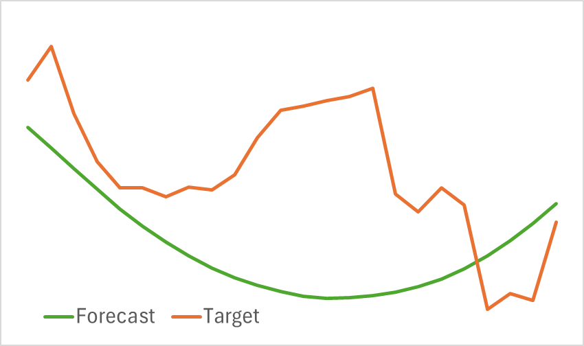
That said, the predicted trajectory is significantly smoothed. The same can be said about the reconstructed trajectory. This indicates considerable noise reduction in the original data. The next stage of model training will determine whether this smoothing is beneficial for developing a profitable Actor policy.
The second stage involves iteratively training the Actor and Critic models. At this stage, we need to find a profitable Actor policy based on the predicted price movement generated by the environmental state encoder. The encoder outputs both forecast and reconstructed historical price movements.
To test the trained models, we used historical data from January 2024 while keeping all other parameters unchanged.
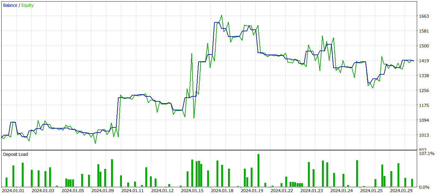
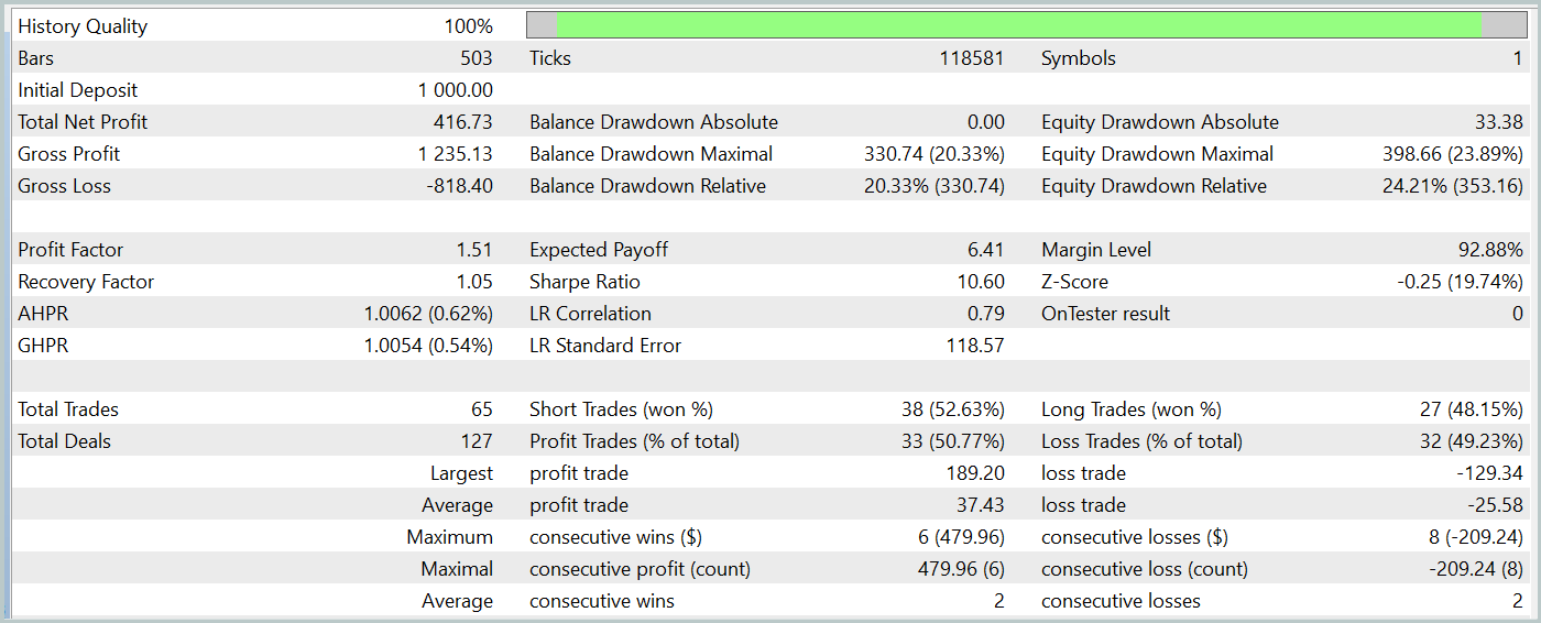
During the test period, our trained Actor model generated over 40% profit with a maximum drawdown of just over 24%. The EA executed a total of 65 trades, 33 of which closed with a profit. Since the maximum and average winning trade values exceed the relevant losing variables, the profit factor was recorded at 1.51. Of course, a one-month test period and 65 trades are insufficient to guarantee long-term stability. However, the results surpass those achieved with the Traj-LLM method.
Conclusion
The UniTraj method presented in this study demonstrates its potential as a versatile tool for processing agent trajectories across various scenarios. This approach addresses a key problem: adapting models to multiple tasks, improving performance compared to traditional methods. Its unified handling of masked input data makes UniTraj a flexible and efficient solution.
In the practical section, we implemented the proposed approaches in MQL5, integrating them into the environmental state Encoder model. We trained and tested the models on real historical data. The obtained results demonstrate the effectiveness of the proposed approaches, which allows them to be used in constructing real-world trading strategies.
References
Programs used in the article
| # | Issued to | Type | Description |
|---|---|---|---|
| 1 | Research.mq5 | EA | Example collection EA |
| 2 | ResearchRealORL.mq5 | EA | EA for collecting examples using the Real-ORL method |
| 3 | Study.mq5 | EA | Model training EA |
| 4 | StudyEncoder.mq5 | EA | Encoder training EA |
| 5 | Test.mq5 | EA | Model testing EA |
| 6 | Trajectory.mqh | Class library | System state description structure |
| 7 | NeuroNet.mqh | Class library | A library of classes for creating a neural network |
| 8 | NeuroNet.cl | Code Base | OpenCL program code library |
Translated from Russian by MetaQuotes Ltd.
Original article: https://www.mql5.com/ru/articles/15648
Warning: All rights to these materials are reserved by MetaQuotes Ltd. Copying or reprinting of these materials in whole or in part is prohibited.
This article was written by a user of the site and reflects their personal views. MetaQuotes Ltd is not responsible for the accuracy of the information presented, nor for any consequences resulting from the use of the solutions, strategies or recommendations described.

- Free trading apps
- Over 8,000 signals for copying
- Economic news for exploring financial markets
You agree to website policy and terms of use