The MQL5 Standard Library Explorer (Part 9): Using ALGLIB to Filter Excessive MA Crossover Signals

MetaTrader 5 — Examples | 4 March 2026, 12:11

601

Clemence Benjamin

Introduction

The Moving Average crossover is probably the first strategy every trader tries. A fast MA crossing above a slow MA signals “buy,” and the reverse signals “sell.” It’s simple, intuitive, and surprisingly effective in trending markets. The problem appears when the market goes sideways: price oscillates around the averages, the lines cross repeatedly, and we get a string of losing trades—the infamous whipsaws.

Many traders attempt to address this by increasing the periods (making the averages smoother but slower) or by adding filters (RSI, ADX, etc.). These approaches can help, but they remain heuristic adjustments layered on top of the original structure.

ALGLIB is a cross-platform numerical analysis library that brings advanced mathematical computing directly into MetaTrader 5 indicators and Expert Advisors. Originally developed for C++, C#, and Python, ALGLIB has been ported to MQL5 as part of the Standard Library distribution, providing us with access to hundreds of optimized algorithms for linear algebra, optimization, signal processing, and data analysis.

For those who might feel intimidated by advanced mathematics, there’s no need to worry. We’ll begin with simple concepts and build gradually. ALGLIB handles the heavy numerical computation internally—we just need to understand what each function does conceptually. Think of it as driving a car: you don’t need to understand thermodynamics to press the accelerator.

In this article, we’ll transform a basic moving average crossover into a mathematically preprocessed system using three ALGLIB techniques:

basic statistical filters,
Singular Spectrum Analysis (SSA),
and spline-based derivative analysis.

By the end, you’ll see how mathematical preprocessing can reduce signal frequency in ranging conditions while preserving responsiveness during trends.

Concept

ALGLIB is a numerical analysis library developed over decades. It provides optimized implementations of algorithms that would take significant time to code from scratch. Within its extensive function set, you’ll find tools for:

Linear algebra—matrix operations, decompositions, equation solvers
Optimization—constrained and unconstrained minimization
Interpolation and fitting—splines, least squares, rational approximations
Data analysis—clustering, principal component analysis
Signal processing—FFT, convolution, filtering
Statistics—distributions, hypothesis testing, correlation analysis

ALGLIB primarily works with specialized structures such as CRowDouble for one-dimensional arrays and CMatrixDouble for matrices. These can be converted to and from native MQL5 vector and matrix types.

Basic Filters (SMA, EMA, LRMA)

ALGLIB provides ready‑to‑use filtering functions that are more efficient and numerically stable than manual implementations. FilterSMA computes a simple moving average using running sums with overflow protection. FilterEMA implements the exponential moving average with precise coefficient handling. FilterLRMA performs linear regression on a sliding window—essentially fitting a straight line to the last K points and returning the value at the current point.

The mathematics behind LRMA is particularly interesting: for each window, it solves a simple linear regression y = a + b*x, where x represents the position within the window. The value at the current point is then a + b*(window‑1). This gives us a filter that responds to linear trends faster than a simple average.

The output value at the most recent point is computed from the regression line, making it more responsive to trends than a simple moving average.

Singular Spectrum Analysis (SSA)

SSA decomposes a time series into structural components such as trend, cycles, and noise. It works by building a trajectory matrix, performing singular value decomposition (SVD), and reconstructing selected components. Conceptually, it separates longer-term structure from short-term fluctuations.

ALGLIB’s CSSAModel manages the process internally by specifying a window size and reconstruction rank.

Spline Interpolation and Derivatives

A cubic spline is a smooth piecewise polynomial passing through data points with continuous first and second derivatives. The first derivative represents the instantaneous rate of change. Zero-crossings of the derivative can indicate directional shifts.

We compare four approaches:

Baseline—EMA crossover on raw prices
Basic filtered—EMA crossover on pre-smoothed prices
SSA filtered—EMA crossover on SSA trend
Spline derivative—zero-crossings as directional cues

By implementing all four in a single indicator, we can visually compare their behavior and see how preprocessing affects signal timing and reliability.

Implementation

Now we’ll build our indicator step by step. Launch MetaEditor, create a new indicator, and let’s dive into the code. We’ll name it ALGLIB_FilterDemo.mq5. This indicator is designed to demonstrate several advanced filtering techniques provided by the ALGLIB numerical library. By applying different filters to the same price series, we can compare their smoothing characteristics and their effect on a simple crossover trading system. The final chart will display multiple lines—each representing a different filtered version of price—along with crossover signals generated from both the raw moving averages and the filtered series.

Step 1: Setting Up the Framework

First, we need to include the ALGLIB library and define our indicator properties. The #include <Math/Alglib/alglib.mqh> directive brings in all the necessary ALGLIB functions for filtering, SSA, splines, and linear algebra. The #property statements set the indicator’s basic behavior: it will be drawn in the main chart window ( indicator_chart_window ), and we allocate ten buffers and ten plots. Allocating ten buffers allows us to store and display the original price, three baseline EMAs (though we only use two for the crossover), five filtered series, and two sets of crossover signals. Having all these lines on the chart at once may seem cluttered, but it gives an immediate visual comparison of how each filter transforms the price data.

//+------------------------------------------------------------------+
//|                                            ALGLIB_FilterDemo.mq5 |
//|                                Copyright 2026, Clemence Benjamin |
//|                                             https://www.mql5.com |
//+------------------------------------------------------------------+
#property copyright "Copyright 2026"
#property link      "https://www.mql5.com"
#property version   "1.00"
#property indicator_chart_window
#property indicator_buffers 10
#property indicator_plots   10

//--- include ALGLIB
#include <Math/Alglib/alglib.mqh>

The indicator_buffers and indicator_plots set to 10 means we’ll have ten lines or markers on our chart. That’s a lot, but we want to see everything at once for comparison.

Step 2: Defining Plot Properties

Each plot needs a label, type, color, and style. We’ll use lines for the continuous series and arrows for crossover signals. The labels will appear in the DataWindow and help identify each line. By assigning distinct colors—black for raw close, blue/red for baseline EMAs, green for SMA‑filtered, dodger blue for EMA‑filtered, orange for LRMA‑filtered, magenta for SSA trend, and brown for the scaled spline derivative—we make the chart readable. Plots 9 and 10 are arrow plots; they will only appear where a crossover occurs, marking potential buy (below the bar) and sell (above the bar) points. The arrow code and empty value will be set later in OnInit.

//--- plot definitions
#property indicator_label1  "Close"
#property indicator_type1   DRAW_LINE
#property indicator_color1  clrBlack
#property indicator_width1  1

#property indicator_label2  "Baseline Fast EMA"
#property indicator_type2   DRAW_LINE
#property indicator_color2  clrBlue
#property indicator_width2  1

#property indicator_label3  "Baseline Slow EMA"
#property indicator_type3   DRAW_LINE
#property indicator_color3  clrRed
#property indicator_width3  1

#property indicator_label4  "SMA Filtered"
#property indicator_type4   DRAW_LINE
#property indicator_color4  clrGreen
#property indicator_width4  1

#property indicator_label5  "EMA Filtered"
#property indicator_type5   DRAW_LINE
#property indicator_color5  clrDodgerBlue
#property indicator_width5  1

#property indicator_label6  "LRMA Filtered"
#property indicator_type6   DRAW_LINE
#property indicator_color6  clrOrange
#property indicator_width6  1

#property indicator_label7  "SSA Trend"
#property indicator_type7   DRAW_LINE
#property indicator_color7  clrMagenta
#property indicator_width7  1

#property indicator_label8  "Spline Derivative (scaled)"
#property indicator_type8   DRAW_LINE
#property indicator_color8  clrBrown
#property indicator_width8  1

#property indicator_label9  "Baseline Crossover Signals"
#property indicator_type9   DRAW_ARROW
#property indicator_color9  clrBlue
#property indicator_width9  1

#property indicator_label10 "Filtered Crossover Signals"
#property indicator_type10  DRAW_ARROW
#property indicator_color10 clrRed
#property indicator_width10 1

Notice that plots 9 and 10 are arrows. We’ll use these to mark buy and sell signals.

Step 3: Input Parameters

We want users to be able to adjust all key parameters. Let’s define them:

//--- input parameters
input int      FastMAPeriod   = 5;           // Fast MA period
input int      SlowMAPeriod   = 20;          // Slow MA period
input int      FilterWindow   = 14;          // Window for SMA/LRMA and EMA alpha (alpha=2/(period+1))
input int      SSAWindow       = 30;          // Window for SSA (must be < data length)
input int      SSARank         = 5;           // Number of SSA components to keep (rank)
input double   SplineDerivScale= 10.0;        // Scaling factor for spline derivative (for visibility)
input int      LookbackBars    = 500;         // Number of recent bars to process (speed optimization)

The LookbackBars parameter is crucial for performance. ALGLIB operations, especially SSA, can be computationally expensive on thousands of bars. By processing only the most recent bars (500 by default), we keep the indicator responsive while still showing plenty of history. Each input parameter controls a specific aspect of the indicator: the baseline crossover uses FastMAPeriod and SlowMAPeriod; FilterWindow determines the length of the simple, exponential, and linear regression moving averages applied to the price; SSAWindow sets the window length for the trajectory matrix in Singular Spectrum Analysis, and SSARank selects how many of the largest eigenvalues are kept for reconstructing the trend; SplineDerivScale simply multiplies the derivative so it becomes visible when plotted; and LookbackBars limits the number of bars fed into the ALGLIB routines.

Step 4: Buffer Declarations

We need ten buffers to hold our data:

//--- indicator buffers
double closeBuffer[];
double baselineFastBuffer[];
double baselineSlowBuffer[];
double smaFilteredBuffer[];
double emaFilteredBuffer[];
double lrmaFilteredBuffer[];
double ssaTrendBuffer[];
double splineDerivBuffer[];
double baselineSignalBuffer[];
double filteredSignalBuffer[];

Each buffer corresponds to one of the plots defined earlier. The closeBuffer holds the raw close prices; baselineFastBuffer and baselineSlowBuffer will be filled by the built‑in iMA function; smaFilteredBuffer, emaFilteredBuffer, and lrmaFilteredBuffer hold the results of applying the respective ALGLIB filters; ssaTrendBuffer stores the SSA‑reconstructed trend; splineDerivBuffer stores the price plus a scaled derivative; and the two signal buffers will hold arrow positions for crossovers. All buffers are declared as dynamic arrays; their sizes will be managed by the terminal.

Step 5: Handles for Built‑in Moving Averages

For the baseline crossover, we’ll use MQL5’s built‑in iMA function. This is already optimized and serves as our reference:

//--- handles for built-in iMA (for baseline)
int fastMAHandle, slowMAHandle;

Using iMA handles is efficient because the terminal calculates the moving averages internally and caches the results. These handles will be created in OnInit and released in OnDeinit.

Step 6: Initialization Function

In OnInit(), we set up our buffers, configure arrow styles, and create the MA handles:

//+------------------------------------------------------------------+
//| Custom indicator initialization function                         |
//+------------------------------------------------------------------+
int OnInit()
{
   //--- set index buffers
   SetIndexBuffer(0, closeBuffer, INDICATOR_DATA);
   SetIndexBuffer(1, baselineFastBuffer, INDICATOR_DATA);
   SetIndexBuffer(2, baselineSlowBuffer, INDICATOR_DATA);
   SetIndexBuffer(3, smaFilteredBuffer, INDICATOR_DATA);
   SetIndexBuffer(4, emaFilteredBuffer, INDICATOR_DATA);
   SetIndexBuffer(5, lrmaFilteredBuffer, INDICATOR_DATA);
   SetIndexBuffer(6, ssaTrendBuffer, INDICATOR_DATA);
   SetIndexBuffer(7, splineDerivBuffer, INDICATOR_DATA);
   SetIndexBuffer(8, baselineSignalBuffer, INDICATOR_DATA);
   SetIndexBuffer(9, filteredSignalBuffer, INDICATOR_DATA);

   //--- set arrow codes (159 = small circle)
   PlotIndexSetInteger(8, PLOT_ARROW, 159);
   PlotIndexSetInteger(9, PLOT_ARROW, 159);
   PlotIndexSetDouble(8, PLOT_EMPTY_VALUE, EMPTY_VALUE);
   PlotIndexSetDouble(9, PLOT_EMPTY_VALUE, EMPTY_VALUE);

   //--- indicator short name
   IndicatorSetString(INDICATOR_SHORTNAME, "ALGLIB Filter Demo (Optimized)");

   //--- get handles for baseline MAs
   fastMAHandle = iMA(_Symbol, _Period, FastMAPeriod, 0, MODE_EMA, PRICE_CLOSE);
   slowMAHandle = iMA(_Symbol, _Period, SlowMAPeriod, 0, MODE_EMA, PRICE_CLOSE);
   if(fastMAHandle == INVALID_HANDLE || slowMAHandle == INVALID_HANDLE)
      return(INIT_FAILED);

   return(INIT_SUCCEEDED);
}

The arrow code 159 gives us a small circle. We set empty values for the signal buffers so they only plot when we explicitly set a value. By assigning INDICATOR_DATA to each buffer, we tell the terminal that these arrays hold the values to be displayed. The handles for the baseline exponential moving averages are created with the user‑selected periods, using the current symbol and timeframe. If either handle fails, the indicator initialization is aborted.

Step 7: Deinitialization

Always release handles when done:

//+------------------------------------------------------------------+
//| Custom indicator deinitialization function                       |
//+------------------------------------------------------------------+
void OnDeinit(const int reason)
{
   if(fastMAHandle != INVALID_HANDLE)  IndicatorRelease(fastMAHandle);
   if(slowMAHandle != INVALID_HANDLE)  IndicatorRelease(slowMAHandle);
}

Releasing the handles is a good practice to free the resources allocated by the terminal. Even though the terminal does this automatically when the indicator is removed, explicit release makes the code robust and portable.

Step 8: Helper Functions for Filters

To keep our code clean, we’ll create helper functions that encapsulate the conversion between MQL5 vectors and ALGLIB’s CRowDouble:

//+------------------------------------------------------------------+
//| Helper to convert vector to CRowDouble and back after filter     |
//+------------------------------------------------------------------+
void ApplySMA(vector<double> &data, int window)
{
   CRowDouble row(data);
   CAlglib::FilterSMA(row, (int)data.Size(), window);
   data = row.ToVector();
}

void ApplyEMA(vector<double> &data, int window)
{
   double alpha = 2.0 / (window + 1.0);
   CRowDouble row(data);
   CAlglib::FilterEMA(row, (int)data.Size(), alpha);
   data = row.ToVector();
}

void ApplyLRMA(vector<double> &data, int window)
{
   CRowDouble row(data);
   CAlglib::FilterLRMA(row, (int)data.Size(), window);
   data = row.ToVector();
}

These functions take a vector by reference, convert it to a CRowDouble, apply the filter, and convert it back. This pattern is essential because ALGLIB works with CRowDouble objects, but we want the convenience of MQL5’s vector type. The functions modify the original vector in‑place, which avoids unnecessary copying and makes the main code more readable. Note that the EMA filter requires the smoothing constant alpha, which is derived from the window length using the standard formula alpha = 2/(period+1) .

Step 9: The Main Calculation Loop

Now for the heart of our indicator—the OnCalculate function. This is where all the ALGLIB magic happens. I’ll break it down section by section.

Determining the Processing Range

First, we decide which bars to process based on LookbackBars:

//+------------------------------------------------------------------+
//| Custom indicator iteration function                              |
//+------------------------------------------------------------------+
int OnCalculate(const int rates_total,
                const int prev_calculated,
                const datetime &time[],
                const double &open[],
                const double &high[],
                const double &low[],
                const double &close[],
                const long &tick_volume[],
                const long &volume[],
                const int &spread[])
{
   //--- Determine the range of bars we need to process
   int startIdx = (rates_total > LookbackBars) ? rates_total - LookbackBars : 0;
   int len = rates_total - startIdx;

This elegant line calculates the starting index. If we have more bars than LookbackBars, we start LookbackBars from the end; otherwise, we start at bar 0. This ensures that we only feed a manageable number of bars into the ALGLIB routines. The length len is the number of bars we will actually process with filters.

Data Validation

We need to ensure we have enough bars for the longest period we’ll use:

   //--- Need enough data for the longest period
   int maxPeriod = MathMax(SlowMAPeriod, MathMax(FilterWindow, SSAWindow));
   if(len < maxPeriod)
   {
      // Not enough bars in the lookback window – fill with EMPTY and return
      for(int i = startIdx; i < rates_total; i++)
      {
         smaFilteredBuffer[i] = EMPTY_VALUE;
         emaFilteredBuffer[i] = EMPTY_VALUE;
         lrmaFilteredBuffer[i] = EMPTY_VALUE;
         ssaTrendBuffer[i]    = EMPTY_VALUE;
         splineDerivBuffer[i] = EMPTY_VALUE;
      }
      ArrayInitialize(baselineSignalBuffer, EMPTY_VALUE);
      ArrayInitialize(filteredSignalBuffer, EMPTY_VALUE);
      return(rates_total);
   }

If the lookback window is too short, we fill everything with empty values and return. This prevents the indicator from plotting partial or incorrect data. The maxPeriod takes the largest of the three key periods (slow MA, filter window, SSA window) to guarantee that all filters have enough data to produce a meaningful output.

Basic Data Copying

We copy close prices to our first buffer (for display) and retrieve the baseline Moving Averages:

   //--- Copy close prices to buffer 0 (for plotting)
   for(int i = 0; i < rates_total; i++)
      closeBuffer[i] = close[i];

   //--- Get baseline MAs (they already cover all bars)
   if(CopyBuffer(fastMAHandle, 0, 0, rates_total, baselineFastBuffer) <= 0) return(0);
   if(CopyBuffer(slowMAHandle, 0, 0, rates_total, baselineSlowBuffer) <= 0) return(0);

The close prices are simply mirrored into the first buffer. The two baseline EMA buffers are filled by copying from the iMA handles. Because these handles contain values for every bar, we copy the entire range. If the copy fails (returns <= 0), we exit early.

Preparing the Data Vector

We create a vector containing only the prices we’ll process:

   //--- Create a vector of close prices for the lookback window
   vector<double> vecClose(len);
   for(int i = 0; i < len; i++)
      vecClose[i] = close[startIdx + i];

This vector, vecClose , holds the price data that will be fed into all the ALGLIB filters. By working on a contiguous segment of the price array, we avoid passing huge arrays and reduce memory and computation overhead.

Applying Basic Filters

Now we apply each filter using our helper functions:

   //--- 1) SMA Filter
   vector<double> vecSMA = vecClose;
   ApplySMA(vecSMA, FilterWindow);
   for(int i = 0; i < len; i++)
      smaFilteredBuffer[startIdx + i] = vecSMA[i];

   //--- 2) EMA Filter
   vector<double> vecEMA = vecClose;
   ApplyEMA(vecEMA, FilterWindow);
   for(int i = 0; i < len; i++)
      emaFilteredBuffer[startIdx + i] = vecEMA[i];

   //--- 3) LRMA Filter
   vector<double> vecLRMA = vecClose;
   ApplyLRMA(vecLRMA, FilterWindow);
   for(int i = 0; i < len; i++)
      lrmaFilteredBuffer[startIdx + i] = vecLRMA[i];

Notice how each filter modifies its own copy of the data. The original vecClose remains unchanged for subsequent operations. The filtered results are then placed into the appropriate buffers at the correct indices ( startIdx + i ). The simple moving average (SMA) gives equal weight to all points in the window; the exponential moving average (EMA) gives more weight to recent prices; and the linear regression moving average (LRMA) fits a straight line to the data and uses the endpoint as the filtered value. These three filters are classic and serve as a baseline for comparison with the more advanced SSA and spline methods.

Singular Spectrum Analysis

This is the most sophisticated part. We create an SSA model, add our data, configure it, and extract the trend:

   //--- 4) SSA Trend
   CSSAModel ssa;
   CAlglib::SSACreate(ssa);
   CRowDouble priceRow(vecClose);                     // convert once
   CAlglib::SSAAddSequence(ssa, priceRow);
   CAlglib::SSASetAlgoTopKRealtime(ssa, SSARank);
   CAlglib::SSASetWindow(ssa, SSAWindow);
   CRowDouble trend, noise;
   CAlglib::SSAAnalyzeLast(ssa, len, trend, noise);

   if(trend.Size() == len)
   {
      vector<double> vecTrend = trend.ToVector();
      for(int i = 0; i < len; i++)
         ssaTrendBuffer[startIdx + i] = vecTrend[i];
   }
   else
   {
      for(int i = 0; i < len; i++)
         ssaTrendBuffer[startIdx + i] = EMPTY_VALUE;
   }

The key line is SSASetAlgoTopKRealtime(ssa, SSARank). This tells SSA to use the top SSARank components (largest eigenvalues) for reconstruction. By keeping only the largest components, we’re essentially filtering out the noise. The window size SSAWindow determines how many past points are considered when building the trajectory matrix—a larger window captures longer‑term patterns but requires more data. After the analysis, we check that the trend has the expected length. If SSA fails (which can happen with insufficient data or numerical issues), we fill with empty values. The resulting trend line should be smoother than any of the simple moving averages and can reveal underlying cyclical components.

Spline Derivative Calculation

For the spline derivative, we need an x‑axis representing bar indices:

   //--- 5) Spline derivative
   // X axis = bar index within the lookback window (0..len-1)
   vector<double> xVec(len);
   for(int i = 0; i < len; i++) xVec[i] = i;

   vector<double> priceVec = priceRow.ToVector();   // already from vecClose

   double xArr[], priceArr[];
   ArrayResize(xArr, len);
   ArrayResize(priceArr, len);
   for(int i = 0; i < len; i++)
   {
      xArr[i] = xVec[i];
      priceArr[i] = priceVec[i];
   }

   CSpline1DInterpolantShell spline;
   CAlglib::Spline1DBuildCubic(xArr, priceArr, len, 0, 0.0, 0, 0.0, spline);

We convert our vectors to plain arrays because Spline1DBuildCubic expects double parameters. The boundary condition parameters (0, 0.0, 0, 0.0) specify a natural cubic spline with zero second derivatives at the ends—a standard choice that works well for most price series. The spline interpolant is then stored in spline .

Now we compute the derivative at each point:

   for(int i = 0; i < len; i++)
   {
      double val, deriv, deriv2;
      CAlglib::Spline1DDiff(spline, i, val, deriv, deriv2);
      splineDerivBuffer[startIdx + i] = close[startIdx + i] + deriv * SplineDerivScale;
   }

We add the scaled derivative to the actual price so the line plots near the price level. Without this shift, the derivative would be near zero and difficult to see. The derivative indicates the rate of change of the smoothed curve; positive values suggest upward momentum, and negative values suggest downward momentum. The scaling factor makes these fluctuations visible as a line that oscillates around the price.

Crossover Signal Detection

Now we generate our trading signals. First, we initialize the signal buffers with empty values:

   //--- 6) Crossover signals (only within lookback window)
   ArrayInitialize(baselineSignalBuffer, EMPTY_VALUE);
   ArrayInitialize(filteredSignalBuffer, EMPTY_VALUE);

For the filtered crossover, we need fast and slow exponential moving averages of the EMA‑filtered series (vecEMA). We’ll compute them recursively into vectors:

   double alphaFast = 2.0 / (FastMAPeriod + 1.0);
   double alphaSlow = 2.0 / (SlowMAPeriod + 1.0);

   vector<double> fastFilteredVec(len);
   vector<double> slowFilteredVec(len);

   if(len > 0)
   {
      fastFilteredVec[0] = vecEMA[0];
      slowFilteredVec[0] = vecEMA[0];
   }
   for(int i = 1; i < len; i++)
   {
      fastFilteredVec[i] = alphaFast * vecEMA[i] + (1 - alphaFast) * fastFilteredVec[i-1];
      slowFilteredVec[i] = alphaSlow * vecEMA[i] + (1 - alphaSlow) * slowFilteredVec[i-1];
   }

This recursive formula is the standard EMA calculation. By precomputing the entire series, we avoid recomputing on each tick and make the code cleaner. Note that we use the same fast and slow periods as the baseline, but apply them to the EMA‑filtered price ( vecEMA ) rather than the raw close. This will produce a crossover signal that is potentially less noisy because the underlying series is already smoothed.

Now we scan for crossovers:

   for(int i = 1; i < len; i++)
   {
      int idx = startIdx + i;

      // Baseline crossover signals (using the built‑in MA buffers)
      if(baselineFastBuffer[idx] > baselineSlowBuffer[idx] && baselineFastBuffer[idx-1] <= baselineSlowBuffer[idx-1])
         baselineSignalBuffer[idx] = low[idx] - 10 * _Point; // buy arrow below price
      if(baselineFastBuffer[idx] < baselineSlowBuffer[idx] && baselineFastBuffer[idx-1] >= baselineSlowBuffer[idx-1])
         baselineSignalBuffer[idx] = high[idx] + 10 * _Point; // sell arrow above price

      // Filtered crossover signals
      if(fastFilteredVec[i] > slowFilteredVec[i] && fastFilteredVec[i-1] <= slowFilteredVec[i-1])
         filteredSignalBuffer[idx] = low[idx] - 20 * _Point; // buy
      if(fastFilteredVec[i] < slowFilteredVec[i] && fastFilteredVec[i-1] >= slowFilteredVec[i-1])
         filteredSignalBuffer[idx] = high[idx] + 20 * _Point; // sell
   }

For buys, we place the arrow below the low of the bar; for sells, above the high. The filtered arrows are placed 20 points away (versus 10 for baseline) so they’re visually distinct. The condition checks for a crossover by comparing the current and previous values of the fast and slow lines. This standard logic generates a signal exactly when the fast line crosses the slow line.

Cleaning Up

Finally, we fill any bars before the lookback window with empty values for the filtered lines:

   //--- Fill any bars before the lookback window with EMPTY_VALUE for the filtered lines
   for(int i = 0; i < startIdx; i++)
   {
      smaFilteredBuffer[i] = EMPTY_VALUE;
      emaFilteredBuffer[i] = EMPTY_VALUE;
      lrmaFilteredBuffer[i] = EMPTY_VALUE;
      ssaTrendBuffer[i]    = EMPTY_VALUE;
      splineDerivBuffer[i] = EMPTY_VALUE;
   }

   //--- return value of prev_calculated for next call
   return(rates_total);
}

And that’s it! Our indicator is complete.

After compiling in MetaEditor, the indicator loads without errors. Applied to USDJPY M15 with default parameters, initialization is efficient due to the LookbackBars optimization. On the chart, you will see the raw close price (black), the two baseline EMA (blue and red), and the five filtered lines (green, dodger blue, orange, magenta, and brown). The blue and red arrows mark crossovers from the baseline EMA, while the red arrows (placed further away) mark crossovers from the filtered EMAs. By comparing the two sets of signals, you can judge whether the additional smoothing helps reduce excessive signals or introduces too much lag.

The implementation includes:

Baseline EMA crossover buffers—the standard fast and slow EMAs calculated by the terminal, providing a familiar reference.
Filtered series buffers (SMA, EMA, LRMA)—three classic moving averages applied via ALGLIB, showing how each smooths the price.
SSA trend reconstruction—a modern, data‑adaptive method that decomposes the series into trend and noise, revealing underlying patterns.
Spline derivative computation—a continuous measure of the smoothed price’s rate of change, scaled for visibility.
Signal visualization logic—two sets of crossover signals (baseline and filtered) plotted as arrows, allowing direct comparison of trade timing and frequency.

Performance optimization focuses on minimizing recalculations and limiting SSA and spline computations to recent bars. The LookbackBars parameter lets you trade off between speed and historical depth. With these building blocks, you can experiment with different filter parameters and even replace the EMA‑filtered crossover with any of the other filtered series to see how they affect signal generation.

Testing

Now that our indicator is compiled successfully, it's time to see it in action. If you're new to this process, don't worry—we'll walk through every step together. The goal here isn't to evaluate profitability (remember, this is a visual tool, not a trading robot). Instead, we want to observe how mathematical preprocessing changes the way moving average crossovers behave—especially during sideways markets.

Step 1: Getting the Indicator on Your Chart

After compiling the code in MetaEditor, the indicator ALGLIB_FilterDemo.ex5 will appear in your Navigator window (View → Navigator or Ctrl+N), inside the "Indicators" folder. If you don't see it, right-click in the Navigator and select "Refresh."

To apply it to a chart:

Open a new chart—we'll use USDJPY, M15 (15-minute) as our example.
Drag the indicator from the Navigator onto the chart, or double-click it.
The indicator's input parameters window will appear. For now, leave everything at its default values:
- Fast MA Period: 5
- Slow MA Period: 20
- Filter Window: 14
- SSA Window: 30
- SSA Rank: 5
- Spline Derivative Scale: 10.0
- Lookback Bars: 500
Click OK.

The indicator will immediately draw several lines on your chart. Don't worry if it looks busy at first—each line has a purpose, and we'll identify them now.

Step 2: Observing the Indicator in Action (Live Chart)

Take a moment to study what appears on your chart. You should see:

Black line: The raw close price (your reference).
Blue and red lines: The baseline fast (5) and slow (20) exponential moving averages—the classic crossover we all know.
Green line: Price filtered with a simple moving average (SMA) using ALGLIB.
Dodger blue line: Price filtered with an exponential moving average (EMA) using ALGLIB.
Orange line: Price filtered with a linear regression moving average (LRMA) using ALGLIB.
Magenta line: The trend component extracted by Singular Spectrum Analysis (SSA).
Brown line: The spline derivative—a measure of the smoothed price's rate of change, scaled and added back to price so it's visible on the chart.
Blue arrows: Crossover signals from the baseline EMAs (placed below bars for buys, above for sells).
Red arrows: Crossover signals from the filtered EMAs (placed slightly further away so they're distinct).

Now, look at a sideways section of the chart—price moving horizontally without a clear trend. Watch what happens:

The baseline EMAs (blue and red) cross back and forth frequently. Each crossing generates a blue arrow. In a ranging market, these arrows will often sometimes appear several in quick succession. This is the "excessive signals" problem we discussed earlier.
Now look at the filtered lines. Notice how the green (SMA), dodger blue (EMA), and orange (LRMA) lines are smoother than the raw price. They don't react to every minor fluctuation.
Pay special attention to the red arrows (filtered crossovers). In that same sideways section, count them. You'll likely see fewer red arrows than blue ones. The preprocessing has filtered out many of the false signals.
The magenta SSA line is often the smoothest of all—it may barely move during sideways periods, producing very few crossovers.
The brown spline derivative line oscillates around price. When it crosses above or below, it signals changes in momentum. You might notice it reacting before the actual crossover occurs—this is the derivative detecting slope changes early.

On live chart

Fig. 1. Live Chart USDJPY M15

Step 3: Testing in the Strategy Tester (Visual Mode)

The live chart shows us recent behavior, but what if we want to see how the indicator performs over a longer historical period—say, several months of data? That's where the Strategy Tester comes in, even though we're not testing an Expert Advisor. We can run the indicator in visual mode to observe its signals across different market conditions.

Here's how to set it up:

Open the Strategy Tester (View → Strategy Tester or Ctrl+R).
In the Tester window:
- Expert Advisor: Leave blank (we're not running an EA).
- Symbol: USDJPY (or any pair you prefer).
- Period: M15.
- Model: Select "Every tick" or "1 minute OHLC" (both work for visual observation).
- Date range: Choose a period that includes both trending and sideways markets—for example, the last 6-12 months.
- Visual mode: Check this box. This is essential—it lets us watch the indicator plot in real-time as the tester runs.
Click "Start." The tester will begin running, and a chart window will open showing the indicator being applied tick by tick or bar by bar.

As the tester runs, observe:

In strong trending periods, both the baseline arrows (blue) and filtered arrows (red) will appear in the same direction. The filtered arrows may appear slightly later (lag is the price of smoothness), but they'll generally align with the trend direction.
In sideways or choppy periods, watch the difference. The blue arrows will fire repeatedly—up, down, up, down—as the fast EMA chases every wiggle. The red arrows, however, will be much sparser. Some sideways sections may produce zero red arrows at all. This is the filtering at work.
Notice how the SSA line (magenta) behaves. During flat periods, it often becomes nearly horizontal, refusing to generate crossovers. It's effectively "sitting out" the noise.
The spline derivative (brown) may still show activity during sideways markets, but. Still, becausee scaled it and added it to the price, its oscillations are visible as wiggles around the price level. You can experiment with the SplineDerivScale parameter to make it more or less pronounced.

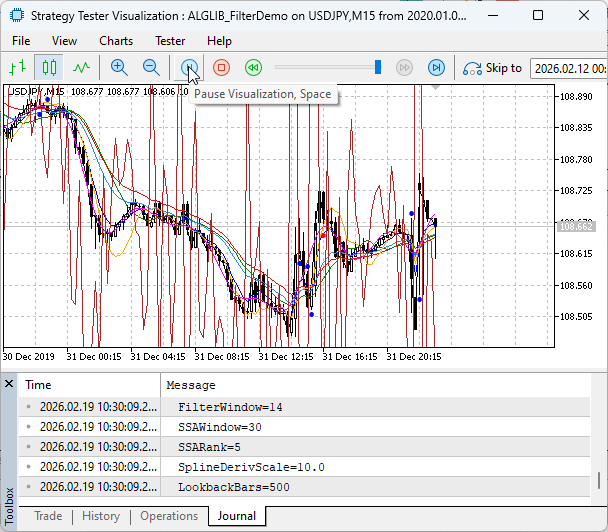
Fig. 2. Strategy Tester Visual Mode

Step 4: Playing with Parameters

One of the best ways to learn is to tweak the inputs and immediately see the effect. Remove the indicator from your chart (right-click → Indicators → select → Delete), then drag it back on and change one parameter at a time. Observe what happens:

Increase FilterWindow (e.g., from 14 to 30): All the filtered lines (green, dodger blue, orange) become smoother. They react more slowly to price changes. Crossover signals (red arrows) will appear less frequently but with more lag. This is the classic trade-off: smoothness vs. responsiveness.
Decrease FilterWindow (e.g., to 5): The filtered lines now hug the raw price more closely. You'll see more red arrows—some may even appear at nearly the same time as blue arrows. The filtering effect is reduced.
Adjust SSAWindow (try 20, then 50): The magenta SSA line changes its smoothness. A smaller window makes it more responsive (but still smoother than raw price); a larger window creates a very slow-moving line that captures only the longest-term movements. If you make the window too large, you may see the line disappear on the left side of the chart—SSA needs enough data to compute.
Change SSARank (try 3, then 8): This controls how many components are kept in the reconstruction. Lower rank = smoother (more aggressive filtering). Higher rank = more detail preserved (closer to original price). Values between 4 and 7 often work well for forex data on M15.
Modify SplineDerivScale: Make it larger (e.g., 20), and the brown line's oscillations become wilder—easier to see, but they may swing far from price. Make it smaller (e.g., 2), and the line hugs price closely, making derivative zero-crossings harder to spot. Find a value that makes the oscillations visible without being distracting.

Through this hands-on experimentation, you'll develop an intuition for how each mathematical technique shapes the data. You're no longer just reading about ALGLIB—you're seeing it work, in real-time, on your own charts.

Conclusion

Now that we've seen the indicator in action—both on live charts and across historical data in the Strategy Tester—let's reflect on what we've accomplished together.

We now have a working indicator that lets us visually compare filtered moving average crossovers side by side. On our charts, we can clearly see how the baseline EMAs behave compared to their filtered counterparts. The filtered crossovers appear less frequently during sideways markets—exactly what we hoped mathematical preprocessing would achieve.

We've learned that we can experiment with parameters to discover how each filter behaves. By adjusting FilterWindow, SSAWindow, SSARank, and SplineDerivScale, we can immediately see the impact on smoothness, lag, and signal frequency. This hands-on exploration builds intuition far better than reading theory alone.

We've seen concrete examples of how mathematics can be applied in trading. The SMA, EMA, and LRMA filters demonstrated familiar smoothing concepts. Singular Spectrum Analysis showed us how data-adaptive decomposition can extract underlying trends. The spline derivative revealed how rate-of-change can be visualized directly on the price chart. None of this required us to become mathematicians—ALGLIB handled the complex calculations while we focused on interpretation.

From a simple moving average crossover, we've built a multi-filter analytical platform. The raw strategy hasn't changed—it's still two moving averages crossing—but the data feeding into it has been transformed. This is the core idea we've explored together: preprocessing matters. The same trading logic applied to differently filtered data produces different signals, and now we have a tool to explore those differences firsthand.

The modular structure of our code means we could:

Replace the EMA-filtered crossover with crossovers from any of the other filtered series (SMA-filtered, LRMA-filtered, SSA trend, etc.) and compare them.
Extract the filtered signals to generate alerts or notifications when crossovers occur.
Use the preprocessing techniques we've demonstrated here as the foundation for an Expert Advisor—taking our filtered crossover logic and automating it for backtesting and forward testing.
Experiment with entirely different ALGLIB functions—optimization routines, clustering algorithms, or advanced statistical tests—and apply them to our trading ideas.

Through this article, we've discovered that ALGLIB transforms MQL5 from a platform limited to built-in indicators into a genuine numerical research environment. Whether we're traders seeking cleaner signals, developers building analytical tools, or simply curious about applied mathematics, ALGLIB opens doors that were previously closed to us.

Download the indicator from the attachment below. Apply it to your favorite pairs and timeframes. Twist the parameters. Break it, fix it, improve it. Let the visual feedback guide your understanding. And when you're ready, take the next step—build that robot, run that optimization, explore that new filter.

I'd love to hear your observations, questions, and experiments in the discussion. The code is yours to use, modify, and learn from. Your contributions help refine these ideas and strengthen our community.

Happy coding, everyone.

Attachments

Source Filename	Type	Version	Description
ALGLIB_FilterDemo	Indicator	1.00	Demonstration indicator showcasing advanced trend filtering techniques using the standard ALGLIB library in MetaTrader 5. It compares traditional EMA crossovers with Linear Regression Moving Average (LRMA) crossovers and includes a cubic spline with derivative-based slope visualization for improved trend detection and reduced whipsaws in ranging markets.

Attached files |

Download ZIP

ALGLIB_FilterDemo.mq5 (12.11 KB)

Warning: All rights to these materials are reserved by MetaQuotes Ltd. Copying or reprinting of these materials in whole or in part is prohibited.

This article was written by a user of the site and reflects their personal views. MetaQuotes Ltd is not responsible for the accuracy of the information presented, nor for any consequences resulting from the use of the solutions, strategies or recommendations described.