Neural Networks in Trading: An Agent with Layered Memory (Final Part)

Introduction

In the previous article, we examined the theoretical foundations of the FinMem framework — an innovative agent based on large language models (LLMs). This framework employs a unique layered memory system that enables efficient processing of data with varying nature and temporal significance.

The FinMem memory module is divided into two main components:

• Working Memory — designed for handling short-term data such as daily news and market fluctuations.
• Long-Term Memory — stores information with lasting value, including analytical reports and research materials.

The stratified memory structure allows the agent to prioritize information, focusing on the data most relevant to current market conditions. For instance, short-term events are analyzed immediately, while deeply impactful information is preserved for future use.

The profiling module of FinMem adapts the agent's behavior to specific professional contexts and market environments. Taking into account the user's individual preferences and risk profile, the agent can optimize its strategy to ensure maximum efficiency in trading operations.

The decision-making module integrates real-time data with stored memories, generating strategies that consider both short-term trends and long-term patterns. This cognitively inspired approach enables the agent to retain key market events and adapt to new signals, significantly enhancing the accuracy and effectiveness of investment decisions.

Experimental results obtained by the framework’s authors demonstrate that FinMem outperforms other autonomous trading models. Even with limited input data, the agent exhibits exceptional efficiency in information processing and strategy formation. Its ability to manage cognitive load allows it to analyze dozens of market signals simultaneously and identify the most critical among them. The agent structures these signals by importance and makes well-founded decisions even under tight time constraints.

Furthermore, FinMem possesses a unique capability for real-time learning, making it highly adaptable to changing market conditions. This allows the agent not only to handle current tasks effectively but also to continually refine its methods as it encounters new data. FinMem combines cognitive principles with advanced technology, offering a modern solution for operating in complex, rapidly evolving financial markets.

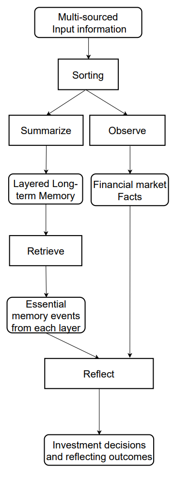
An author-provided visualization of the FinMem framework's information flow is shown below.

In the previous article, we began implementing the approaches proposed by the framework’s authors using MQL5, and introduced our own interpretation of the layered memory module CNeuronMemory, which differs significantly from the original version. In our FinMem implementation, we deliberately excluded the large language model — a key component of the initial concept. This inevitably influenced all parts of the system.

Despite this, we made every effort to reproduce the framework's core information flows. In particular, the CNeuronFinMem object was designed to preserve the stratified approach to data processing. This object successfully integrates methods for handling short-term information and long-term strategies, ensuring stable and predictable performance in dynamic market environments.

Building the FinMem Framework

Recall that we previously stopped at building the integrated algorithm of the proposed framework within the CNeuronFinMem object, the structure of which is shown below.

class CNeuronFinMem   :  public CNeuronRelativeCrossAttention
  {
protected:
   CNeuronTransposeOCL  cTransposeState;
   CNeuronMemory        cMemory[2];
   CNeuronRelativeCrossAttention cCrossMemory;
   CNeuronRelativeCrossAttention cMemoryToAccount;
   CNeuronRelativeCrossAttention cActionToAccount;
   //---
   virtual bool      feedForward(CNeuronBaseOCL *NeuronOCL) override   { return false; }
   virtual bool      feedForward(CNeuronBaseOCL *NeuronOCL, CBufferFloat *SecondInput) override;
   virtual bool      calcInputGradients(CNeuronBaseOCL *NeuronOCL) override   { return false; }
   virtual bool      calcInputGradients(CNeuronBaseOCL *NeuronOCL, CBufferFloat *SecondInput, 
                     CBufferFloat *SecondGradient, ENUM_ACTIVATION SecondActivation = None) override;
   virtual bool      updateInputWeights(CNeuronBaseOCL *NeuronOCL) override   { return false; }
   virtual bool      updateInputWeights(CNeuronBaseOCL *NeuronOCL, CBufferFloat *SecondInput) override;

public:
                     CNeuronFinMem(void) {};
                    ~CNeuronFinMem(void) {};
   //---
   virtual bool      Init(uint numOutputs, uint myIndex, COpenCLMy *open_cl,
                          uint window, uint window_key, uint units_count, uint heads,
                          uint accoiunt_descr, uint nactions,
                          ENUM_OPTIMIZATION optimization_type, uint batch);
   //---
   virtual int       Type(void) override   const   {  return defNeuronFinMem; }
   //---
   virtual bool      Save(int const file_handle) override;
   virtual bool      Load(int const file_handle) override;
   //---
   virtual bool      WeightsUpdate(CNeuronBaseOCL *source, float tau) override;
   virtual void      SetOpenCL(COpenCLMy *obj) override;
   //---
   virtual bool      Clear(void) override;
  };

Earlier, we discussed the initialization of the object. Now, we will move on to constructing the feed-forward method, which takes two primary parameters.

The first parameter is a tensor — a multidimensional data array representing the state of the environment. It contains various market data such as current quotes and values of analyzed technical indicators. This approach allows the model to account for a broad spectrum of variables, enabling decision-making based on a comprehensive analysis.

The second parameter is a vector containing information about the trading account state. It includes the current balance, profit and loss data, and a timestamp. This component ensures real-time data availability and supports accurate calculations.

bool CNeuronFinMem::feedForward(CNeuronBaseOCL *NeuronOCL, CBufferFloat *SecondInput)
  {
   if(!cTransposeState.FeedForward(NeuronOCL))
      return false; 

To perform a comprehensive analysis of the environment state, we begin by processing the initial data represented as a multidimensional tensor. The transposition procedure transforms the array, making it easier to work with different projections for a more detailed extraction of key characteristics.

Next, two projections of the input data are passed into specialized memory modules for in-depth analysis. The first module focuses on studying the temporal dynamics of market parameters organized as bars, allowing the model to capture and interpret the complex behavior of the analyzed financial instrument. The second module concentrates on analyzing unitary sequences of multimodal time series, enabling the detection of hidden dependencies between indicators and capturing their correlations. This creates an integrated representation of the current market state.

Such an analytical structure ensures a high level of accuracy and provides flexible adaptation of the model to changing market dynamics — a crucial factor for achieving reliable and timely financial decisions.

   if(!cMemory[0].FeedForward(NeuronOCL) ||
      !cMemory[1].FeedForward(cTransposeState.AsObject()))
      return false;

The results from both memory modules are combined using a cross-attention block, which enriches multimodal time series with insights derived from the analysis of univariate sequences. This enhances both the precision and completeness of the resulting information, making it more suitable for informed decision-making.

   if(!cCrossMemory.FeedForward(cMemory[0].AsObject(), cMemory[1].getOutput()))
      return false;

Next, we examine the impact of market changes on account balance. To achieve this, the results of the multi-level market analysis are compared with the account state vector through a cross-attention module. This methodological approach allows for more accurate assessment of how market events influence financial metrics. The analysis helps identify complex dependencies between market activity and financial outcomes. This is especially important for forecasting and risk management.

   if(!cMemoryToAccount.FeedForward(cCrossMemory.AsObject(), SecondInput))
      return false;

The next step involves the operational decision-making block. Here, the model compares the Agent's most recent actions with the corresponding profits and losses to determine their interdependencies. At this stage, we assess the efficiency of the current policy and whether it requires adjustment. This approach prevents repetitive patterns and increases the flexibility of the trading strategy — particularly valuable in high-volatility conditions.

Additionally, the model can evaluate the acceptable risk level for the next trading operation.

It is important to note that the tensor of the Agent's recent actions serves as the third data source. However, we remember that the method supports processing only two input data streams. So, we take advantage of the fact that the Agent's action tensor is generated as the output of this very object and remains stored in its result buffer until the next feed-forward operation. This allows us to call the feed-forward pass of the internal cross-attention block using a pointer to the current object, similar to recurrent modules.

   if(!cActionToAccount.FeedForward(this.AsObject(), SecondInput))
      return false;

At this point, we must ensure that the tensor of the Agent's latest actions is preserved until it is replaced with new data — this guarantees correct execution of backpropagation operations. To achieve this, we replace data buffer pointers accordingly, minimizing the risk of information loss.

   if(!SwapBuffers(Output, PrevOutput))
      return false;

After that, we invoke the parent class method, responsible for generating a new Agent action tensor. This process is based on the analytical results obtained earlier within the current method. As a result, a continuous chain of interactions between different modules is maintained, ensuring high data consistency and relevance.

   if(!CNeuronRelativeCrossAttention::feedForward(cActionToAccount.AsObject(), cMemoryToAccount.getOutput()))
      return false;
//---
   return true;
  }

The method concludes by returning the logical result of the operation to the calling program.

The constructed feed-forward algorithm exhibits a nonlinear nature, which significantly affects data handling during the backpropagation phase. This is particularly evident in the gradient distribution algorithm implemented in the calcInputGradients method. To execute this process correctly, information must be processed strictly in reverse order, mirroring the logic of the feed-forward pass. This requires accounting for all unique architectural characteristics of the model to ensure computational accuracy and consistency.

In the parameters of the calcInputGradients method, we receive pointers to the two input data stream objects, to which we will transmit the error gradients according to each stream’s contribution to the model’s final output.

bool CNeuronFinMem::calcInputGradients(CNeuronBaseOCL *NeuronOCL,
                                       CBufferFloat *SecondInput,
                                       CBufferFloat *SecondGradient,
                                       ENUM_ACTIVATION SecondActivation = -1)
  {
   if(!NeuronOCL || !SecondInput || !SecondGradient)
      return false;

In the method body, we immediately check if the received pointers are relevant. Without this, further operations are meaningless, as gradient propagation would be impossible.

Recall that the feed-forward phase concluded with a call to the parent class method, responsible for the final stage of processing. Accordingly, gradient backpropagation begins with the corresponding method of the parent class. Its task is to propagate the gradient across two internal cross-attention blocks of parallel data-processing paths.

   if(!CNeuronRelativeCrossAttention::calcInputGradients(cActionToAccount.AsObject(),
         cMemoryToAccount.getOutput(),
         cMemoryToAccount.getGradient(),
         (ENUM_ACTIVATION)cMemoryToAccount.Activation()))
      return false;

It is important to note that along one of these data pathways, we recursively used the results of the previous feed-forward pass of our object as input data. This creates a continuous loop during backpropagation, which now must be broken.

To correctly distribute the error gradient, we must first restore the buffer with results from the previous feed-forward pass, which were used as input for the cross-attention module analyzing their relationship with the financial outcome. This is achieved by substituting the relevant buffer pointers, allowing the data to be restored without loss and with minimal overhead.

   if(!SwapBuffers(Output, PrevOutput))
      return false;

In addition, we must also replace the pointer to the object's gradient buffer to preserve data obtained from the subsequent layer. For this, we use any available buffer of sufficient size. Naturally, the environment-state tensor is much larger than the Agent's action vector. So, we can use one of the buffers from that data stream.

   CBufferFloat *temp = Gradient;
   if(!SetGradient(cMemoryToAccount.getPrevOutput(), false))
      return false;

Once all critical data are secured, we call the gradient distribution method through the cross-attention block that analyzes the effect of prior agent actions on the obtained financial result.

   if(!calcHiddenGradients(cActionToAccount.AsObject(), SecondInput, SecondGradient, SecondActivation))
      return false;

Afterward, we restore all buffer pointers to their original state.

   if(!SwapBuffers(Output, PrevOutput))
      return false;
   Gradient = temp;

At this point, we have distributed the error gradient along the Agent action evaluation path. We have passed the corresponding gradients to both the memory stream and the account state vector buffer. However, note that the account-state buffer participates in two data flows: the memory and the Agent's action paths. We have already propagated the gradient along the latter. Now, we must determine the influence of the account-state data on the model's final output through the memory path and then sum the gradients obtained from both flows.

   if(!cCrossMemory.calcHiddenGradients(cMemoryToAccount.AsObject(), SecondInput, cMemoryToAccount.getPrevOutput(),
                                                                                                 SecondActivation))
      return false;
   if(!SumAndNormilize(SecondGradient, cMemoryToAccount.getPrevOutput(), SecondGradient, 1, false, 0, 0, 0, 1))
      return false;

Next, we continue distributing the error gradient along the memory pathway down to the level of the original input data, according to their impact on the model's output. Here, again, we deal with two projections of the input data. We first distribute the gradient through these two analytical streams.

   if(!cMemory[0].calcHiddenGradients(cCrossMemory.AsObject(), cMemory[1].getOutput(), cMemory[1].getGradient(),
                                                                      (ENUM_ACTIVATION)cMemory[1].Activation()))
      return false;

And then propagate it down to the data transposition object.

   if(!cTransposeState.calcHiddenGradients(cMemory[1].AsObject()))
      return false;

At this stage, we must transmit the error gradient to the original input data object from both parallel memory streams. First, we propagate the errors along one stream.

   if(!NeuronOCL.calcHiddenGradients(cMemory[0].AsObject()))
      return false;

then replace the data buffers and propagate the gradient along the second.

   temp = NeuronOCL.getGradient();
   if(!NeuronOCL.SetGradient(cTransposeState.getPrevOutput(), false) ||
      !NeuronOCL.calcHiddenGradients(cTransposeState.AsObject()) ||
      !NeuronOCL.SetGradient(temp, false) ||
      !SumAndNormilize(temp, cTransposeState.getPrevOutput(), temp, iWindow, false, 0, 0, 0, 1))
      return false;
//---
   return true;
  }

Finally, we sum the gradients from both information flows and restore all buffer pointers to their original state. The method then returns a logical result to the calling program, marking the end of its execution.

This concludes our examination of the algorithms used to construct the methods of the CNeuronFinMem object. You can find the complete code of this class and all its methods in the attachment.

Model Architecture

We have completed the implementation of the FinMem framework approaches in MQL5 within the CNeuronFinMem object. This implementation provides the basic functionality and serves as a foundation for further integration with learning algorithms. The next step is to integrate the created object into the trainable Agent model, which serves as the core decision-making component in financial systems. The architecture of this trainable model is defined within the CreateDescriptions method.

It should be noted that the FinMem framework goes beyond purely architectural design. It also includes unique learning algorithms that enable the model to adapt and efficiently process data in complex financial environments. However, we will return to the learning process later. For now, it is important to emphasize that we will train only one model: the Agent.

In the parameters of the CreateDescriptions method, we receive a pointer to a dynamic array used to store the structure of the model being created.

bool CreateDescriptions(CArrayObj *&actor)
  {
//---
   CLayerDescription *descr;
//---
   if(!actor)
     {
      actor = new CArrayObj();
      if(!actor)
         return false;
     }

Inside the method, we immediately verify the validity of the received pointer and, if necessary, create a new instance of the dynamic array.

Next, we create the data preprocessing block. This block includes a fully connected layer that receives the raw input data, followed by a batch normalization layer that reduces the model's sensitivity to data scale variations and improves training stability. This approach ensures the efficient performance of the subsequent model components.

//--- Actor
   actor.Clear();
//--- Input layer
   if(!(descr = new CLayerDescription()))
      return false;
   descr.type = defNeuronBaseOCL;
   int prev_count = descr.count = (HistoryBars * BarDescr);
   descr.activation = None;
   descr.optimization = ADAM;
   if(!actor.Add(descr))
     {
      delete descr;
      return false;
     }
//--- layer 1
   if(!(descr = new CLayerDescription()))
      return false;
   descr.type = defNeuronBatchNormOCL;
   descr.count = prev_count;
   descr.batch = 1e4;
   descr.activation = None;
   descr.optimization = ADAM;
   if(!actor.Add(descr))
     {
      delete descr;
      return false;
     }

Following this block comes the FinMem module we developed earlier, which serves as the foundation for implementing the key aspects of data processing and decision formation.

//--- layer 2
   if(!(descr = new CLayerDescription()))
      return false;
   descr.type = defNeuronFinMem;
//--- Windows
     {
      int temp[] = {BarDescr, AccountDescr, 2*NActions}; //Window, Account description, N Actions
      if(ArrayCopy(descr.windows, temp) < int(temp.Size()))
         return false;
     }
   descr.count = HistoryBars;
   descr.window_out = 32;
   descr.step = 4;                              // Heads
   descr.batch = 1e4;
   descr.activation = None;
   descr.optimization = ADAM;
   if(!actor.Add(descr))
     {
      delete descr;
      return false;
     }

In the windows array, we define three main tensor dimensions for the input data: the description of a single bar, the account state, and the agent's actions. The latter also represents the dimensionality of the block's output vector.

It is worth noting that in this case, the dimension of the Agent's action tensor is set to twice the corresponding constant. This approach allows us to implement the stochastic head mechanism for the Agent. As is customary, the first half represents the mean values of the distributions, while the second half corresponds to their variances. Accordingly, it is important to recall that when initializing cross-attention objects working with the Agent's action tensor, we divided the main input stream into two equal vectors. This enables the block to produce consistent pairs of means and variances at its output.

The generation of values within these defined distributions is handled by the latent-state layer of a variational autoencoder.

//--- layer 3
   if(!(descr = new CLayerDescription()))
      return false;
   descr.type = defNeuronVAEOCL;
   descr.count = NActions;
   descr.optimization = ADAM;
   if(!actor.Add(descr))
     {
      delete descr;
      return false;
     }

Finally, the architecture concludes with a convolutional layer, which projects the obtained values into the required action range for the Agent.

//--- layer 4
   if(!(descr = new CLayerDescription()))
      return false;
   descr.type = defNeuronConvSAMOCL;
   descr.count = NActions / 3;
   descr.window = 3;
   descr.step = 3;
   descr.window_out = 3;
   descr.activation = SIGMOID;
   descr.optimization = ADAM;
   descr.probability = Rho;
   if(!actor.Add(descr))
     {
      delete descr;
      return false;
     }
//---
   return true;
  }

All that remains is to return the result of the operations to the calling program and exit the method.

Training Program

We have made significant progress in implementing the approaches proposed by the authors of the FinMem framework. At this stage, we already have a model architecture capable of effectively processing financial data and adapting to complex market conditions. A distinctive feature of the developed model is its layered memory, simulating human-like cognitive processes.

As mentioned earlier, the authors of the framework proposed not only architectural principles but also a training algorithm based on a layered approach to data processing. This allows the model to capture not only linear relationships but also complex nonlinear dependencies between parameters. During training, the model accesses a wide spectrum of data from multiple sources, enabling the formation of a comprehensive representation of the financial environment. This, in turn, enhances adaptability to changing market conditions and improves forecast accuracy.

When a training request with analyzed data is received, the model activates two key processes: observation and generalization. The system observes market labels, which include daily price changes of the analyzed financial instrument. These labels serve as indications of "Buy" or "Sell" actions. This information allows the model to identify and prioritize the most relevant memories, ranking them based on extraction scores from each layer of long-term memory.

Meanwhile, the long-term memory component of FinMem retains critical data for future use — key events and memories. They are processed at deeper memory levels to ensure durable storage. Repeated trading operations and market reactions reinforce the relevance of stored information, contributing to the continuous improvement of decision quality.

Our earlier decision to exclude the large language model (LLM) from the implementation also affects the training process. Nevertheless, we strive to preserve the original learning principles proposed by the framework authors. In particular, during training, we will allow the model to "look into the future", similar to approaches used in price movement forecasting models. However, there is an important nuance here. In this case, we cannot simply provide the model with future price movement data. The output of our model consists of parameters of a trading operation. So, during training, we must supply similar data as feedback (training labels). Therefore, during training, based on the available information about upcoming price movements, we will attempt to generate an almost ideal trading decision as a reference.

Let us now look at how this proposed approach is implemented in code. In this article, we will focus only on the training method Train. The full training program can be found in the attached file: "...\Experts\FinMem\Study.mq5".

The beginning of the model training method is fairly conventional: we generate a vector of trajectory-selection probabilities from the experience replay buffer, based on the profitability of stored runs, and declare the necessary local variables.

void Train(void)
  {
//---
   vector<float> probability = GetProbTrajectories(Buffer, 0.9);
//---
   vector<float> result, target, state;
   matrix<float> fstate = matrix<float>::Zeros(1, NForecast * BarDescr);
   bool Stop = false;

Next, we organize the training loop. However, in this case, we are dealing with recurrent models, which are sensitive to the order of input data. Therefore, we have to use nested loops. In the outer loop, we sample one trajectory from the experience replay buffer along with its initial state. In the inner loop, we sequentially iterate through the states along the selected trajectory. The number of training iterations and the batch size are defined in the external parameters of the training program.

   for(int iter = 0; (iter < Iterations && !IsStopped() && !Stop); iter += Batch)
     {
      int tr = SampleTrajectory(probability);
      int start = (int)((MathRand() * MathRand() / MathPow(32767, 2)) * (Buffer[tr].Total - 2 - NForecast - Batch));
      if(start <= 0)
        {
         iter -= Batch;
         continue;
        }
      if(!Actor.Clear())
        {
         PrintFormat("%s -> %d", __FUNCTION__, __LINE__);
         Stop = true;
         break;
        }
      for(int i = start; i < MathMin(Buffer[tr].Total, start + Batch); i++)
        {
         if(!state.Assign(Buffer[tr].States[i].state) ||
            MathAbs(state).Sum() == 0 ||
            !bState.AssignArray(state))
           {
            iter -= Batch + start - i;
            break;
           }

It is crucial to note that before starting training on a new trajectory, we must clear the model's memory. Because the stored data must correspond to the environment currently being analyzed.

Inside the inner loop, we first extract the description of the analyzed environment state from the replay buffer and form the account state vector.

It is important to emphasize that here we form the account state vector, rather than just transferring it from the experience buffer as before. Previously, we simply reformatted and passed along the stored information. Now, however, we must account for the fact that the model learns to analyze the impact of the Agent's previous actions on the obtained financial result. Consequently, the account state vector must depend on these actions, which cannot be achieved by a simple data transfer from the buffer.

The first step is to generate the harmonics of the timestamp corresponding to the analyzed environment state.

         bTime.Clear();
         double time = (double)Buffer[tr].States[i].account[7];
         double x = time / (double)(D'2024.01.01' - D'2023.01.01');
         bTime.Add((float)MathSin(x != 0 ? 2.0 * M_PI * x : 0));
         x = time / (double)PeriodSeconds(PERIOD_MN1);
         bTime.Add((float)MathCos(x != 0 ? 2.0 * M_PI * x : 0));
         x = time / (double)PeriodSeconds(PERIOD_W1);
         bTime.Add((float)MathSin(x != 0 ? 2.0 * M_PI * x : 0));
         x = time / (double)PeriodSeconds(PERIOD_D1);
         bTime.Add((float)MathSin(x != 0 ? 2.0 * M_PI * x : 0));
         if(bTime.GetIndex() >= 0)
            bTime.BufferWrite();

We also retrieve the vector of the Agent's most recent actions stored in the model buffer.

         //--- Previous Action
         Actor.getResults(result);

The we compute the return of that action as the price change during the last bar of the analyzed environment state. I must admit that, to simplify the algorithm, we use a basic return calculation. We do not account for events such as stop-loss or take-profit triggers, nor for possible commissions on trades. Furthermore, it is assumed that all previously opened positions were closed before the Agent's last operation. This approach is acceptable for a rough evaluation of the model's performance, but before using it in live trading all market specifics and related parameters must be taken into account in detail.

To compute the return of the last operation, we simply multiply the price change by the difference between buy and sell volumes from the vector of the Agent's recent actions:

         float profit = float(bState[0] / (_Point * 10) * (result[0] - result[3]));

Recall that we take the price change as the difference between close and open prices. Therefore, we have a positive value for a bullish candle and a negative value otherwise. The difference in trade volumes likewise gives a positive number for buy operations and a negative one for sell operations. Consequently, the product of these two values produces the correct signed result for the trade.

Next, we extract from the experience replay buffer the balance and equity data of the prior state — the state in which the trading operation proposed by the Agent on the previous step was intended to be executed.

         //--- Account
         float PrevBalance = Buffer[tr].States[MathMax(i - 1, 0)].account[0];
         float PrevEquity = Buffer[tr].States[MathMax(i - 1, 0)].account[1];

As noted earlier, we assume that all previously opened positions were closed before executing new trades. This implies that the balance is adjusted to the equity level.

         bAccount.Clear();
         bAccount.Add((PrevEquity - PrevBalance) / PrevBalance);

The equity change over the last trading bar equals the financial result of the last trading operation calculated above.

         bAccount.Add((PrevEquity + profit) / PrevEquity);
         bAccount.Add(profit / PrevEquity);

We execute the trade only for the volume difference, which is reflected in the open positions metrics.

         bAccount.Add(MathMax(result[0] - result[3], 0));
         bAccount.Add(MathMax(result[3] - result[0], 0));

Accordingly, we report the financial result only for the open position.

         bAccount.Add((bAccount[3]>0 ? profit / PrevBalance : 0));
         bAccount.Add((bAccount[4]>0 ? profit / PrevBalance : 0));
         bAccount.Add(0);
         bAccount.AddArray(GetPointer(bTime));
         if(bAccount.GetIndex() >= 0)
            bAccount.BufferWrite();

After preparing the input data, we perform a feed-forward pass through our model, during which a new vector of Agent actions will be produced.

         //--- Feed Forward
         if(!Actor.feedForward((CBufferFloat*)GetPointer(bState), 1, false, GetPointer(bAccount)))
           {
            PrintFormat("%s -> %d", __FUNCTION__, __LINE__);
            Stop = true;
            break;
           }

Now, to perform backpropagation, we need to prepare target values for the "ideal" trading operation based on information about the upcoming price movement. For this, we extract from the experience replay buffer the data for the specified planning horizon.

         //--- Look for target
         target = vector<float>::Zeros(NActions);
         bActions.AssignArray(target);
         if(!state.Assign(Buffer[tr].States[i + NForecast].state) ||
            !state.Resize(NForecast * BarDescr) ||
            MathAbs(state).Sum() == 0)
           {
            iter -= Batch + start - i;
            break;

Reformat them into a matrix.

         if(!fstate.Resize(1, NForecast * BarDescr) ||
            !fstate.Row(state, 0) ||
            !fstate.Reshape(NForecast, BarDescr))
           {
            iter -= Batch + start - i;
            break;
           }

Then we reorder the rows of the matrix so that the data follow chronological order.

         for(int i = 0; i < NForecast / 2; i++)
           {
            if(!fstate.SwapRows(i, NForecast - i - 1))
              {
               PrintFormat("%s -> %d", __FUNCTION__, __LINE__);
               Stop = true;
               break;
              }
           }

The first column of our forecast matrix contains price changes per bar. We take the cumulative sum of these values to obtain the total price change at each step of the forecast period.

         target = fstate.Col(0).CumSum();

Note that this approach does not account for potential gaps. Given the relatively low probability of such events in our experiments, we are willing to neglect them for now. However, this simplification is unacceptable when preparing real trading decisions.

The further formation of the target Agent action vector depends on the prior operation. If a position was open on the previous step, we search for an exit point. Consider the exit algorithm for a long trade as an example. First, we determine the set stop-loss level and declare the necessary local variables.

         if(result[0] > result[3])
           {
            float tp = 0;
            float sl = 0;
            float cur_sl = float(-(result[2] > 0 ? result[2] : 1) * MaxSL * Point());
            int pos = 0;

Then we iterate through the forecasted price values searching for the point where the current stop-loss is hit. During the iteration we record maximum and minimum values in order to set new stop-loss and take-profit levels.

            for(int i = 0; i < NForecast; i++)
              {
               tp = MathMax(tp, target[i] + fstate[i, 1] - fstate[i, 0]);
               pos = i;
               if(cur_sl >= target[i] + fstate[i, 2] - fstate[i, 0])
                  break;
               sl = MathMin(sl, target[i] + fstate[i, 2] - fstate[i, 0]);
              }

In the case of downward movement, the take-profit value will naturally remain "0", which will produce a zero action vector. This will result in closing all open positions and waiting for the next bar to open.

If an upward movement is expected, a new Agent action vector is generated specifying adjusted trading level values.

            if(tp > 0)
              {
               sl = float(MathMin(MathAbs(sl) / (MaxSL * Point()), 1));
               tp = float(MathMin(tp / (MaxTP * Point()), 1));
               result[0] = MathMax(result[0] - result[3], 0.01f);
               result[1] = tp;
               result[2] = sl;
               for(int i = 3; i < NActions; i++)
                  result[i] = 0;
               bActions.AssignArray(result);
              }
           }

The vector for exiting a short position is formed likewise.

         else
           {
            if(result[0] < result[3])
              {
               float tp = 0;
               float sl = 0;
               float cur_sl = float((result[5] > 0 ? result[5] : 1) * MaxSL * Point());
               int pos = 0;
               for(int i = 0; i < NForecast; i++)
                 {
                  tp = MathMin(tp, target[i] + fstate[i, 2] - fstate[i, 0]);
                  pos = i;
                  if(cur_sl <= target[i] + fstate[i, 1] - fstate[i, 0])
                     break;
                  sl = MathMax(sl, target[i] + fstate[i, 1] - fstate[i, 0]);
                 }
               if(tp < 0)
                 {
                  sl = float(MathMin(MathAbs(sl) / (MaxSL * Point()), 1));
                  tp = float(MathMin(-tp / (MaxTP * Point()), 1));
                  result[3] = MathMax(result[3] - result[0], 0.01f);
                  result[4] = tp;
                  result[5] = sl;
                  for(int i = 0; i < 3; i++)
                     result[i] = 0;
                  bActions.AssignArray(result);
                 }
              }

A slightly different approach is used when no position is open. In that case we first determine the nearest dominant trend.

               ulong argmin = target.ArgMin();
               ulong argmax = target.ArgMax();
               while(argmax > 0 && argmin > 0)
                 {
                  if(argmax < argmin && target[argmax] > MathAbs(target[argmin]))
                     break;
                  if(argmax > argmin && target[argmax] < MathAbs(target[argmin]))
                     break;
                  target.Resize(MathMin(argmax, argmin));
                  argmin = target.ArgMin();
                  argmax = target.ArgMax();
                 }

The action vector is then formed in accordance with that trend. The trade volume is set at the minimum lot per each 100 USD of the current balance.

               if(argmin == 0 || argmax < argmin)
                 {
                  float tp = 0;
                  float sl = 0;
                  float cur_sl = - float(MaxSL * Point());
                  ulong pos = 0;
                  for(ulong i = 0; i < argmax; i++)
                    {
                     tp = MathMax(tp, target[i] + fstate[i, 1] - fstate[i, 0]);
                     pos = i;
                     if(cur_sl >= target[i] + fstate[i, 2] - fstate[i, 0])
                        break;
                     sl = MathMin(sl, target[i] + fstate[i, 2] - fstate[i, 0]);
                    }
                  if(tp > 0)
                    {
                     sl = (float)MathMin(MathAbs(sl) / (MaxSL * Point()), 1);
                     tp = (float)MathMin(tp / (MaxTP * Point()), 1);
                     result[0] = float(Buffer[tr].States[i].account[0] / 100 * 0.01);
                     result[1] = tp;
                     result[2] = sl;
                     for(int i = 3; i < NActions; i++)
                        result[i] = 0;
                     bActions.AssignArray(result);
                    }
                 }
               else
                 {
                  if(argmax == 0 || argmax > argmin)
                    {
                     float tp = 0;
                     float sl = 0;
                     float cur_sl = float(MaxSL * Point());
                     ulong pos = 0;
                     for(ulong i = 0; i < argmin; i++)
                       {
                        tp = MathMin(tp, target[i] + fstate[i, 2] - fstate[i, 0]);
                        pos = i;
                        if(cur_sl <= target[i] + fstate[i, 1] - fstate[i, 0])
                           break;
                        sl = MathMax(sl, target[i] + fstate[i, 1] - fstate[i, 0]);
                       }
                     if(tp < 0)
                       {
                        sl = (float)MathMin(MathAbs(sl) / (MaxSL * Point()), 1);
                        tp = (float)MathMin(-tp / (MaxTP * Point()), 1);
                        result[3] = float(Buffer[tr].States[i].account[0] / 100 * 0.01);
                        result[4] = tp;
                        result[5] = sl;
                        for(int i = 0; i < 3; i++)
                           result[i] = 0;
                        bActions.AssignArray(result);
                       }
                    }
                 }
              }
           }

Having formed the vector of "near-ideal" actions, we perform the backward pass of our model, minimizing the deviation between the agent’s predicted actions and our target values.

         //--- Actor Policy
         if(!Actor.backProp(GetPointer(bActions), (CBufferFloat*)GetPointer(bAccount), GetPointer(bGradient)))
           {
            PrintFormat("%s -> %d", __FUNCTION__, __LINE__);
            Stop = true;
            break;
           }

Now we only need to inform the user about the training progress and proceed to the next iteration of our nested loop system.

         if(GetTickCount() - ticks > 500)
           {
            double percent = double(iter + i - start) * 100.0 / (Iterations);
            string str = StringFormat("%-14s %6.2f%% -> Error %15.8f\n", "Actor", percent,
                                                           Actor.getRecentAverageError());
            Comment(str);
            ticks = GetTickCount();
           }
        }
     }

After successfully completing all iterations of the training loop, we clear the comment field on the instrument chart that was used to inform the user. We log the training results and initiate the program shutdown procedure.

   Comment("");
//---
   PrintFormat("%s -> %d -> %-15s %10.7f", __FUNCTION__, __LINE__, "Actor", Actor.getRecentAverageError());
   ExpertRemove();
//---
  }

This concludes our examination of the algorithms used to build the FinMem framework in MQL5. The complete source code for all presented objects, their methods, and the programs used to prepare this article is available in the attachment for your review.

Testing

The last two articles focused on the FinMem framework. In them, we implemented our interpretation of the approaches proposed by the framework authors using MQL5. We have now reached the most exciting stage: evaluating the effectiveness of the implemented solutions on real historical data.

It is important to emphasize that during the implementation we made significant modifications to the FinMem algorithms. Consequently, we assess only our implemented solution, not the original framework.

The model was trained on historical data for the EURUSD currency pair for 2023 using the H1 timeframe. Indicator settings analyzed by the model were left at their default values.

For the initial training phase we used a dataset formed during previous research. The implemented training algorithm, which generates "near-ideal" target actions for the Agent, allows training the model without updating the training dataset. However, to cover a broader range of account states, I would recommend adding periodic updates to the training dataset where possible.

After several training cycles we obtained a model that demonstrated stable profitability on both training and test data. Final testing was carried out on historical data for January 2024 with all other parameters unchanged. The test results are presented below.

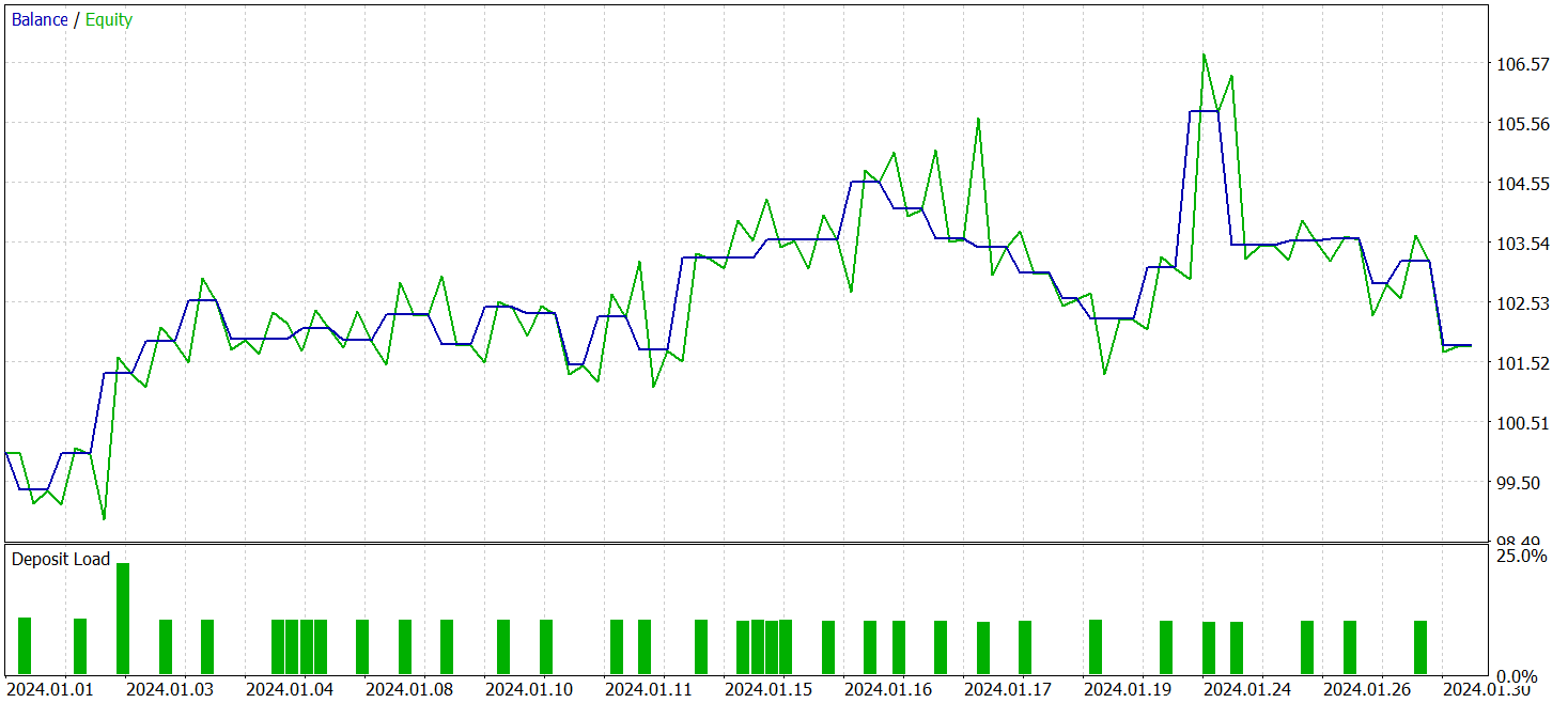
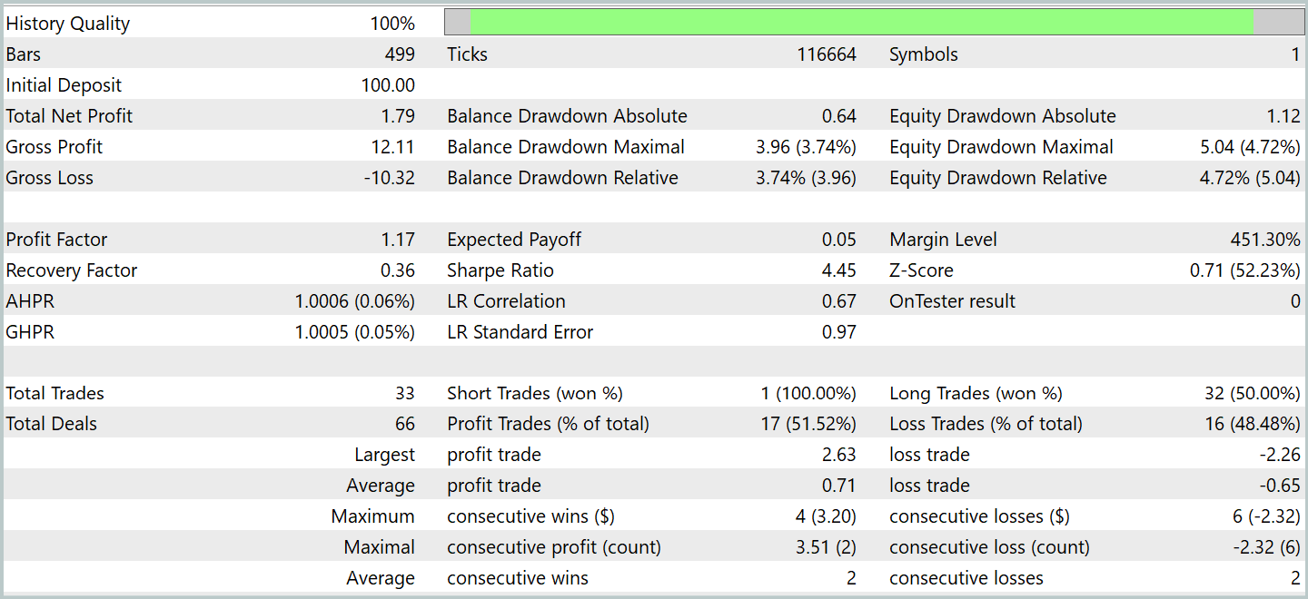
During the testing period the model executed 33 trades, of which slightly more than half were closed with profit. The average and maximum profitable trade exceeded the corresponding metrics for losing trades, enabling the model to show a balance-growth tendency. This indicates the potential of the proposed approaches and their feasibility for use in live trading.

Conclusion

We explored the FinMem framework, which represents a new stage in the evolution of autonomous trading systems. The framework combines cognitive principles with modern algorithms based on large language models. Layered memory and real-time adaptability enable the agent to make reasoned and accurate investment decisions even in unstable market conditions.

In the practical part of this work we implemented our own interpretation of the proposed approaches using MQL5, while omitting the large language model. The results of the experiments confirm the effectiveness of the proposed approaches and their applicability in real trading. Nevertheless, for full deployment on live financial markets the model requires additional tuning and training on a more representative dataset, accompanied by thorough comprehensive testing.

References

• FinMem: A Performance-Enhanced LLM Trading Agent with Layered Memory and Character Design
• Other articles from this series

Programs used in the article

#	Name	Type	Description
1	Research.mq5	Expert Advisor	Expert Advisor for collecting samples
2	ResearchRealORL.mq5	Expert Advisor	Expert Advisor for collecting samples using the Real-ORL method
3	Study.mq5	Expert Advisor	Model training EA
4	Test.mq5	Expert Advisor	Model Testing Expert Advisor
5	Trajectory.mqh	Class library	System state and model architecture description structure
6	NeuroNet.mqh	Class library	A library of classes for creating a neural network
7	NeuroNet.cl	Code library	OpenCL program code