Building a Trading System (Part 5): Managing Gains Through Structured Trade Exits

Introduction

In the previous article, we explored how variations in win-rate could emerge from the same trade entry confirmation. We observed that even when a trader identifies a valid entry, the eventual results may differ significantly depending on how the trade is managed. Much of this variation arises not from the entry itself, but from the exit strategy—whether the trade is cut short, left to run, or subjected to mechanical stop adjustments such as trailing stops.

This raises an important point: in trading, the difference between long-term profitability and long-term frustration often lies not in the quality of entries, but in the discipline of exits.

For many beginners and even experienced traders, trade management is an emotional battlefield. Common experiences include:

• Watching a trade come within a few points of the take-profit target, only to reverse sharply and hit the stop-loss.
• Seeing a trade close at breakeven due to a tightly set trailing stop, only for the market to later surge in the original direction and surpass the original target. Exiting prematurely due to fear of loss, only to miss out on a larger move that unfolds afterwards.

Each of these scenarios highlights the chaotic nature of financial markets. Unlike controlled laboratory experiments, trading outcomes are heavily influenced by volatility spikes, sudden liquidity changes, news events, and random noise. 

“The markets are a place where you can do everything right and still lose, and do everything wrong and still win.”

This paradox is both humbling and enlightening. It teaches us that a trader’s job is not to seek perfect prediction, but rather to build structured systems that can navigate chaos over the long run.

So, how can we build a strategy that mitigates these common frustrations? This article focuses on using multiple entries at different Reward-to-Risk Ratios (RRR) to systematically secure gains and reduce overall risk exposure. We will delve into the mathematical foundation of this approach and outline a plan to test it using a Monte Carlo simulation.

How Traders Secure Their Gains

So, how do traders avoid those painful experiences we talked about earlier? How can they make sure their profits don’t just appear — but actually stay?

Over the years, traders have come up with many techniques, but most of them fall into three broad categories.

1. Trailing Stops — Letting Profits Breathe, Not Escape

A trailing stop is like a safety net that moves with your trade. As the market moves in your favor, the stop level follows — locking in profits while still allowing room for further growth.

Used well, it’s one of the simplest and most effective ways to protect gains and automate risk management. But it’s not foolproof. Set the trailing distance too tight, and you’ll get stopped out before the trade has room to develop. Make it too wide, and it loses its protective value.

Some traders refine this by using volatility-based trailing stops, like ATR multiples, to let the system adapt to changing market conditions. Still, as we saw in Part 4, this doesn’t eliminate randomness entirely — results can remain uneven.

2. Partial Lot Reductions — Taking Something Off the Table

Another popular approach is the partial closure method — a way to “have your cake and eat it too.”

Here’s how it works: a trader opens a full-sized position, and once the market moves favorably, closes part of it to secure some profits. For instance, after opening 3 lots, they might reduce exposure to 2 lots once a certain target is reached.

This early gain brings psychological relief — the sense that the trade is already a winner — while the remaining position keeps them in the game for potential further upside.

The key challenge? Discipline. Without a clear plan for when and how much to reduce, the trader risks locking in too little or too much, turning what could have been a balanced strategy into guesswork.

3. Multiple Entries with Varying Reward-to-Risk Ratios — Structuring the Chaos

The third method takes the logic of partial closures and turns it into a systematic framework. Instead of one position being scaled out, the trader opens multiple positions at once, each with:

• the same stop-loss,
• butdifferent profit targets, based on specific Reward-to-Risk Ratios (RRR).

Imagine five trades, targeting RRR values of 1.3, 1.4, 1.5, 1.6, and 1.7. As the price progresses, each target locks in profits step by step, building a layered structure of realized gains.

This technique spreads risk across outcomes, creates measurable consistency, and aligns with probability-based expectancy. It’s not without its demands — you’ll need precise position sizing and discipline in risk allocation — but when executed well, it can transform market noise into something structured, testable, and even optimizable.

Each of these methods aims at the same goal — turning potential gains into secured results — but they do it in very different ways. Whether you prefer the automation of trailing stops, the flexibility of partial closures, or the structure of multiple entries, the key lies in consistency and discipline.

Because in trading, it’s not just about making profits — it’s about keeping them.

Mathematical Framework

Let's illustrate this with a clear example. Assume we execute 5 trades simultaneously from the same entry. The first trade has an RRR of 1.3, and each subsequent trade's RRR increases by 0.1. We assume a fixed stop-loss of 50 pips for all trades.

The potential outcomes for this basket of trades are as follows:

Scenario	Wins	Losses	Wins -Losses	Net Outcome (in RRR)	Net Outcome (in Pips)
Worst Case	0	5	(0-5)	-5 R	-250 pips
Poor Case	1	4	(1.3- 4)	-2.7 R	-135 pips
Near-Breakeven	2	3	(1.3 + 1.4 - 3)	-0.3 R	-15 pips
Profitable	3	2	(1.3 + 1.4 + 1.5 - 2)	+2.2 R	+110 pips
Very Profitable	4	1	(1.3 + 1.4 + 1.5 + 1.6 - 1)	+4.8 R	+240 pips
Ideal Case	5	0	(1.3 + 1.4 + 1.5 + 1.6 + 1.7)	+7.5 R	+375 pips

Key Insight: With this specific RRR progression, you only need 3 out of 5 trades to be profitable. However, even with only 2 wins, the total loss is minimal (-15 pips) compared to the full loss of -250 pips if you had traded a single position. This demonstrates a powerful reduction in risk exposure.

Monte Carlo Simulation: Bridging Theory and Reality

Mathematics provides clarity, but trading is never linear. Random sequences of wins and losses create unexpected equity curves. To evaluate how this multiple-entry method holds up in reality, we turn to Monte Carlo simulations.

Monte Carlo methods simulate thousands of random trade sequences to mimic the chaos of live markets. Our simulation will compare three scenarios for a trading system with a fixed 3% total risk per trade:

• Single Trade: One trade with a fixed RRR.
• Two Trades: Two simultaneous trades with different RRRs, each risking 1.5% (total 3%).
• Three Trades: Three simultaneous trades with different RRRs, each risking 1% (total 3%).

We will evaluate these under different win-rates, such as 43% (low accuracy system) with initial RRR=1.3, and 65% (high accuracy system) with initial RRR=0.9. This allows us to compare expectancy, risk distribution, and drawdowns across strategies.

Case Study

Case 1: A system with 43% win-rate at RRR=1.3

We conducted a Monte Carlo simulation using an initial equity of $1,000, a 43% win-rate system, and a base RRR of 1.3.

The simulation was run under three trading strategies:

• Single Trade per Execution (RRR = 1.3)
• Two Trades per Execution (RRRs = 1.3 and 1.5)
• Three Trades per Execution (RRRs = 1.3, 1.5, and 1.7)

For both the two-trade and three-trade setups, we introduced a step increment of rstep = 0.2, which allowed progressive scaling of RRR levels across entries. For each scenario, 100 Monte Carlo iterations were performed. The results highlight key differences in equity growth, drawdowns, and profitability distribution across the three strategies.

• Scenario 1: Single Trade Execution

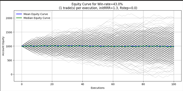
Figure 1: 43% Win-rate for single trade per execution

Table 1: 43% Win-rate Single Entry

Metrics	Values
Risk per trade%	3%
Mean Equity Curve	$986.00
Median Equity Curve	$967.00
Median Drawdown %	30.23%
Profitable %	48.60%

Key Insight:

The single-trade approach struggles under a 43% win-rate system. With mean equity falling below the starting balance, the expectancy is negative. Nearly half of the Monte Carlo runs (48.6%) ended profitable, but drawdowns averaged above 30%, signaling significant risk to capital stability.

This confirms the challenge of running a system with limited accuracy at a fixed RRR: the margin for error is too thin, and equity erosion becomes likely.

• Scenario 2: Two Trade Execution

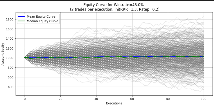
Figure 2: 43% Win-rate for two trades per execution

Table 2: 43% Win-rate Double Entry

Metrics	Values
Risk per trade%	1.5%
Mean Equity Curve	$1,026.00
Median Equity Curve	$1,021.00
Median Drawdown %	22.50%
Profitable %	52.20%

Key Insight:

By splitting the trade into two entries at different RRRs (1.3 and 1.5), performance improves notably. The mean and median equity values now rise above $1,000, indicating positive expectancy.

Drawdowns are also reduced by almost one-third compared to Scenario 1 (22.5% vs. 30.2%), while the proportion of profitable runs climbs above 50%. This shows that the distribution of exits across two RRR levels cushions the system against streaks of losses and provides a smoother equity curve.

• Scenario 3: Three Trade Execution

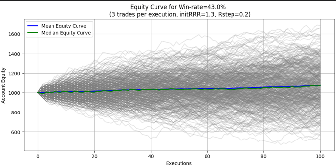
Figure 3: 43% Win-rate for three trades per execution

Table 3: 43% Win-rate Triple Entry

Metrics	Values
Risk per trade%	1%
Mean Equity Curve	$1,071.00
Median Equity Curve	$1,072.00
Median Drawdown %	17.14%
Profitable %	61.80%

Key Insight:

The three-trade strategy delivers the strongest results. Both mean and median equity levels are significantly higher than the starting balance, with an average gain of over 7% after the simulations.

Most importantly, risk stability improves: median drawdowns fall to just 17.1% (a nearly 50% reduction from Scenario 1). The probability of finishing profitable also rises sharply to 61.8%, making this approach far more resilient in the face of randomness.

This demonstrates that spreading exposure across multiple RRR targets not only increases expectancy but also reduces volatility of returns—a dual benefit that enhances long-term sustainability.

Comparative Analysis

Table 4: 43% win-rate analysis

Strategy	Mean Equity	Median Equity	Median Drawdown	Profitable %	Key Takeaway
1 Trade (RRR=1.3)	$986.00	$967.00	30.23%	48.60%	Negative expectancy; high drawdowns
2 Trades (1.3,1.5)	$1,026.00	$1,021.00	22.50%	52.20%	Positive expectancy; reduced drawdown
3 Trades (1.3,1.5,1.7)	$1,071.00	$1,072.00	17.14%	61.80%	Strongest results; higher profits, lower risk

Case 2: A system with 65% win-rate at RRR=0.9

In this scenario, we examined a trading system with a relatively strong win-rate of 65% and an initial RRR of 0.9. Unlike the earlier scenario with lower probability of success, here the high win-rate changes the dynamics of profitability and drawdown control. To fully explore its performance, we evaluated the system under three distinct strategies:

• Single Tradeper Execution (RRR = 0.9 )
• Two Tradesper Execution(RRR = 0.9 and 1.1, rstep = 0.2)
• Three Tradesper Execution(RRR = 0.9, 1.1, and 1.3, rstep = 0.2)

Each configuration was subjected to 100 independent simulations, and the key outcomes: equity progression, drawdown, and probability of profitability, were compared.

• Scenario 4: Single Trade Execution

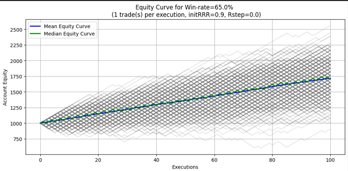
Figure 4: 65% Win-rate for single trade per execution

Table 5: 65% Win-rate Single Entry

Metrics	Values
Risk per trade%	3%
Mean Equity Curve	$1,716.00
Median Equity Curve	$1,705.00
Median Drawdown %	10.24%
Profitable %	99.80%

Key Insight:

The single-trade configuration demonstrated reliable profitability across simulations, with nearly every run finishing in profit (99.8%). The median equity curve outcome of $1,705 indicates consistent growth compared to the $1,000 starting balance. However, the trade-off is the relatively higher drawdown of 10.24%, a natural consequence of concentrating full risk on one position. While this strategy ensures simplicity, it exposes the account to deeper equity fluctuations.

• Scenario 5: Two Trade Execution

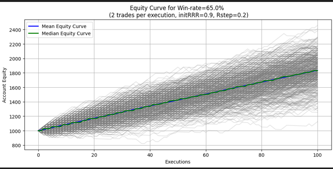
Figure 5: 65% Win-rate for two trades per execution

Table 6: 65% Win-rate Double Entry

Metrics	Values
Risk per trade%	1.5%
Mean Equity Curve	$1,834.00
Median Equity Curve	$1,831.00
Median Drawdown %	5.69%
Profitable %	100.00%

Key Insight:

Shifting to two simultaneous trades transformed the risk-return profile. By splitting the 3% total risk into two smaller positions, the system achieved better balance between reward capture and drawdown control. The median equity curve rose significantly to $1,831, and the median drawdown dropped nearly by half, to 5.69%. Every single simulation closed profitably, suggesting that diversification across two reward levels (RRR = 0.9 and 1.1) provides both stability and resilience.

This demonstrates the power of risk distribution: the same total risk produces higher equity growth with less volatility when allocated across multiple trades.

• Scenario 6: Three Trade Execution

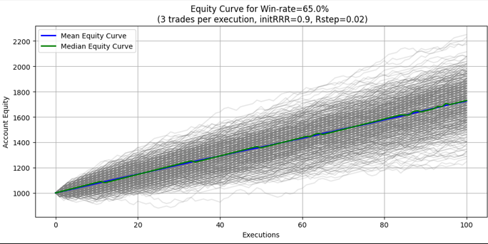
Figure 6: 65% Win-rate for three trades per execution

Table 7: 65% Win-rate Triple Entry

Metrics	Values
Risk per trade%	1%
Mean Equity Curve	$1,953.00
Median Equity Curve	$1,959.00
Median Drawdown %	3.98%
Profitable %	100.00%

Key Insight:

The three-trade system represents the most balanced and robust configuration. With positions distributed across three reward levels (RRR = 0.9, 1.1, and 1.3), the results showed clear superiority in both growth and stability. The median equity curve reached $1,959, the highest of all strategies, while median drawdown declined further to 3.98%, the lowest risk exposure observed.

Most importantly, the probability of profitability reached 100%, making this configuration exceptionally reliable across repeated simulations. The synergy of diversification, high win-rate, and progressive RRR scaling ensured consistently positive outcomes with minimal downside risk.

Comparative Analysis

Table 8: 65% win-rate analysis

Strategy	Mean Equity	Median Equity	Median Drawdown	Profitable %	Key Takeaway
1 Trade (RRR=0.9)	$1,716.00	$1,705.00	10.24%	99.80%	Strong expectancy; low drawdowns
2 Trades (0.9, 1.1)	$1,834.00	$1,831.00	5.69%	100.00%	Improved returns; smoother equity curve
3 Trades (0.9, 1.1, 1.3)	$1,953.00	$1,959.00	3.98%	100.00%	Best performance; highest profits, lowest risk

RRR Increment (rstep) Sensitivity

The RRR increment (rstep) is a critical determinant of profitability or loss in multi-trade strategies.

• If rstep is set too high, the gap between profit targets widens. While this can yield larger wins on higher RRR trades, it often reduces the probability that all targets are reached.
• If rstep is set too low, profit levels cluster too closely, limiting overall gains and reducing the efficiency of diversification.

The key insight is that rstep must be aligned with the system’s win-rate and minimum RRR threshold for profitability. When the system’s win-rate is above the breakeven RRR, rstep adjustments ensure that no profit level falls significantly below this threshold, preserving expectancy.

Sensitivity Test: 43% Win-Rate System (rstep = 0.3)

We re-ran the simulations for the 43% win-rate system, increasing rstep from 0.2  to 0.3. The same base conditions applied (initial RRR = 1.3, total risk = 3%).

Table 9: 43% win-rate rtsep sensitivity test

Strategy	Mean Equity	Median Equity	Median Drawdown	Profitable %	Key Takeaway
2 Trades (1.3, 1.6)	$1,054,00	$1,048.00	21.59%	56.60%	Larger RRR spread improves expectancy modestly
3 Trades (1.3, 1.6,1.9)	$1,126.00	$1,125.00	16.08%	71.20%	Strong gains and lower risk; outperform rstep = 0.2

Key Insight:

• Equity Growth – Increasing rstep to 0.3 yielded higher mean and median equity than with 0.2 (e.g., 3 trades rose from $1,070.57 → $1,125.83).
• Risk Management – Median drawdown improved slightly with larger rstep, dropping to 16.08% under the 3-trade system.
• Profitability Probability – A wider rstep increased profitable outcomes to 71.20%, versus 61.8% under rstep = 0.2.
• Optimal Range – Moderate rstep widening (0.3) proved beneficial in this case, but excessively high increments could reduce reliability if win-rate is low.

Monte Carlo Simulation Code

The following parameters define the structure of the Monte Carlo simulation, allowing traders to test different scenarios and observe the range of possible outcomes based on their system’s backtest statistics:

# Simulation parameters
win_rate = 0.43 # 43%
initial_rrr = 1.3  # reward-risk-ratio
rrr_step = 0.2   # rrr increment
risk_percent = 0.01  # 1% risk per trade
num_executions = 100   # Number of confirmation for entry
trades_per_execution = 3   # number of trade per execution
simulations = 500    # number of simulation runs
initial_balance = 1000   # starting balance

• win-rate: The historical probability of a trade ending in profit. In this case, the system wins 43% of its trades.
• initial_rrr: The base RRR for the first trade. A value of 1.3 means the profit target is 1.3 times the size of the stop-loss.
• rrr_step: The incremental increase in RRR between trades when using multiple entries. For example, if the first trade is 1.3 RRR, the next would target 1.5, and the third 1.7.
• risk_percent:  The fraction of account equity risked per trade. Here, each trade risks 1% of the balance.
• num_executions: The number of times entry signals (trade confirmations) are executed in a single simulation run.
• trades_per_execution:  The number of trades placed simultaneously per execution. In this example, each execution opens 3 trades at different profit targets.
• simulations: The total number of Monte Carlo runs performed. Running many simulations helps capture the range of possible outcomes, smoothing out randomness.
• initial_balance: The starting account equity. All results (profits, losses, drawdowns) are measured relative to this baseline.

Demonstration: Executing Multiple Trades at Different Take Profit Levels

To make the multi-trade strategy practical, we provide a script file designed to help traders automatically open multiple orders at different take profit (TP) levels. This script eliminates the manual effort of calculating and placing several orders, ensuring that trades are executed consistently with your chosen parameters.

Input Settings Explained

The script comes with configurable input settings, allowing traders to customize their execution style as shown in Figure 7.

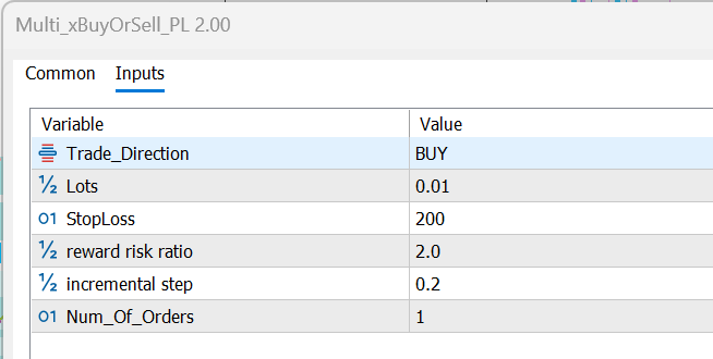
Figure 7: Input settings

1. Trade_Direction: Defines whether the script opens buy or sell trades. Default: Buy
2. Lots: Sets the lot size for each order. All trades opened in a batch use the same lot size. Default: 0.01
3. Stoploss: Determines the stop-loss distance (in points). Protects capital by capping losses on each trade. Default: 200 points (20 pips)
4. Reward-to-Risk Ratio (RRR): Sets the profit target as a multiple of the stop-loss. Default: 2 (i.e., profit target is 2× stop-loss) 
5. Increment Step (rstep): Defines the distance between one take profit level and the next. Larger increments spread profit targets further apart, while smaller increments cluster them closer together.
6. Number of Orders: Specifies how many trades to open per execution. Each trade will be assigned a unique TP based on the increment step. Default: 1 trade

How It Works

The script opens several trades at once, each sharing the same stop-loss but targeting progressively higher profit levels. By splitting the trade into multiple segments, traders can secure profits at earlier levels while still keeping part of the position active for larger gains. This approach provides both risk management (locking in gains early) and growth potential (capturing extended moves).

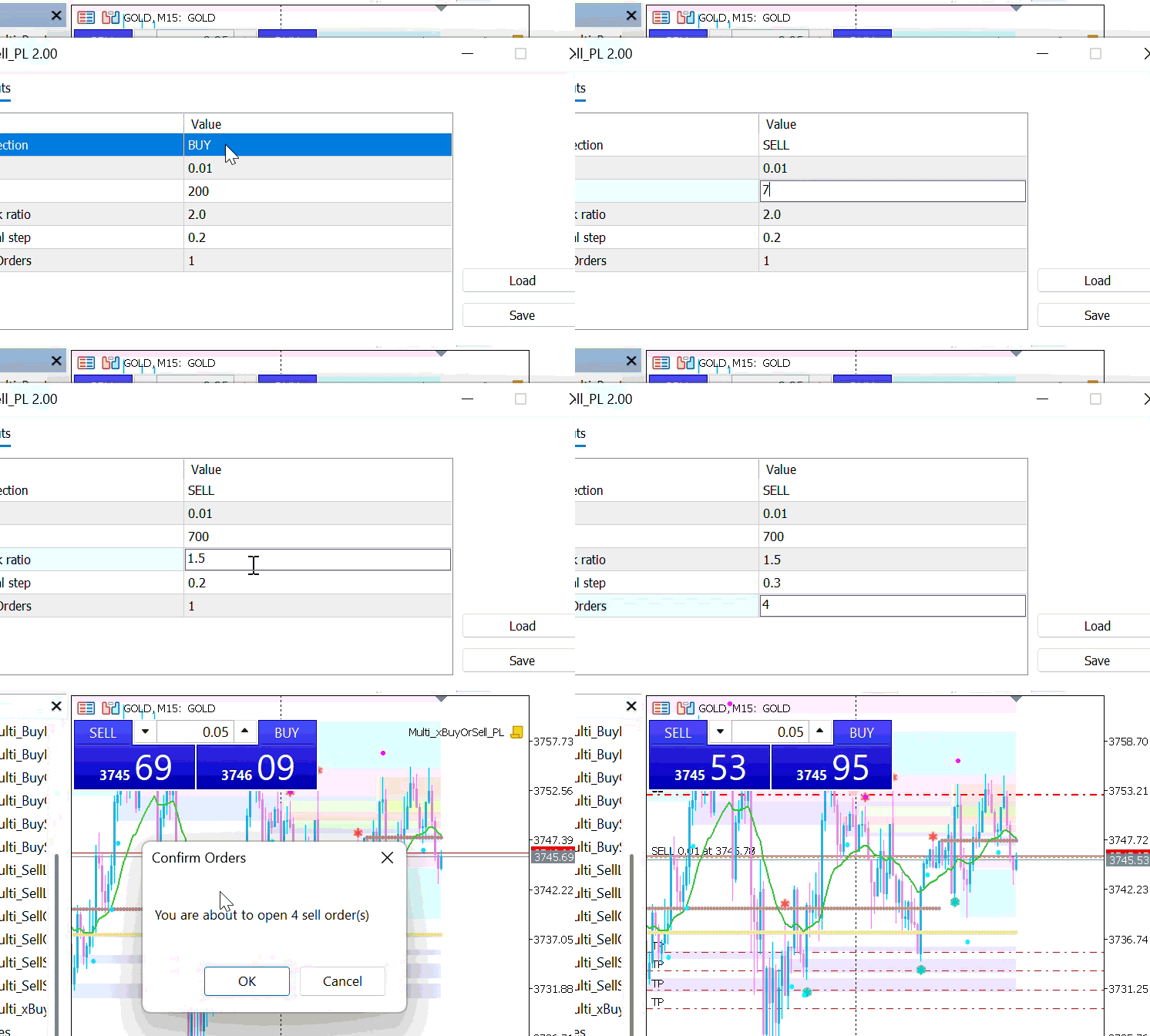
Figure 8: Multi_Sell Demonstration

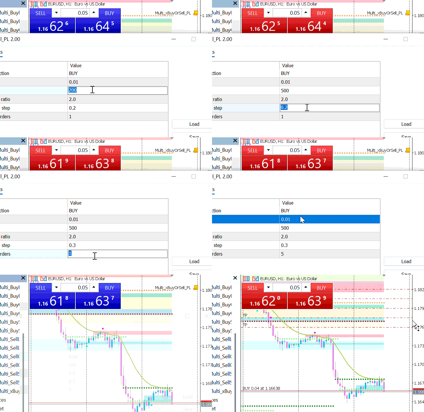
Figure 9: Multi_Buy Demonstration

Recommendation

Adopt Multi-Trade Structures

• For systems with lower win-rates (below 50%), split entries into 2–3 trades with gradually increasing RRR levels.
• This cushions losses, improves expectancy, and reduces drawdowns compared to single-trade strategies.

Keep Total Risk Fixed

• Fix a total risk budget (e.g., 3% per trade setup) and redistribute it across multiple trades rather than increasing overall risk exposure.
• This ensures stability and prevents equity erosion during losing streaks.

Optimize RRR Increments (rstep)

• Avoid setting rstep too small (profit targets cluster, limiting gains) or too large (profit targets become unrealistic).
• As shown, moderate increments (e.g., 0.3 for a 43% win-rate system) enhance profitability and stability.

Leverage Simulation Tools

• Use Monte Carlo simulations or backtesting frameworks to stress-test strategies under different win-rates, RRR levels, and rsteps.
• This helps validate robustness before committing real capital.

Conclusion

This study highlights that the structure of trade execution and profit-taking design is just as important as entry confirmation. Through Monte Carlo simulations, we demonstrated how varying win-rates, RRR, and rstep shape both profitability and risk exposure.

For the 43% win-rate system, a single-trade approach consistently underperformed, producing negative expectancy and high drawdowns. However, splitting risk across multiple trades with incrementally higher RRR levels (2- or 3-trade strategies) improved outcomes significantly—reducing drawdowns, lifting equity curves, and raising the probability of profitability. Further, sensitivity testing on rstep showed that widening profit levels (from 0.2 to 0.3) enhanced performance, especially under the 3-trade configuration.

In contrast, the 65% win-rate system demonstrated robust profitability across all strategies. Here, the single-trade model was already strong, but diversification into 2- and 3-trade structures smoothed equity curves, reduced drawdowns to below 4%, and locked in a 100% probability of profitability.

The overarching insight is that:

• Low to moderate win-rate systems benefit most from multiple entries and carefully tuned rstep values. Diversification helps convert marginally negative expectancy into positive performance.
• High win-rate systems are inherently profitable but can be made more stable by spreading risk across tiers.
• Risk allocation discipline is critical. Keeping total risk fixed (e.g., 3%) while redistributing across multiple trades creates resilience without sacrificing upside.

Ultimately, the results emphasize that traders should not only focus on finding “perfect entries” but must also engineer execution frameworks that maximize expectancy while minimizing downside volatility. A robust system is not defined by a single setup but by how intelligently risk, reward, and probability are balanced over the long run.

Final Note

Through this series on Building a Trading Systems, the aim has been to show that success in the markets requires more than just finding good entries—it demands structure, discipline, and adaptability. By exploring win-rates, reward-to-risk ratios, multiple trade executions, Monte Carlo simulations, and sensitivity to RRR increments, we have demonstrated practical ways to design more robust and resilient systems.

I hope researchers, traders, and system developers alike have gained valuable insights to guide their journey toward consistency. While there is always more to learn and refine, the concepts shared here provide a foundation that—when combined with practice and testing—can build both confidence and skill in navigating the chaos of the markets.

Trading will always involve uncertainty, but with a strong framework, the odds shift in your favor. Continue testing, refining, and adapting your strategies, and remember: the goal is not perfection, but long-term resilience and steady growth.

Until then, trade smart, stay disciplined, and happy trading!