
Build Self Optimizing Expert Advisors in MQL5 (Part 7): Trading With Multiple Periods At Once

Technical indicators present the modern investor with many opportunities and equivalent challenges. There are many well-known limitations of technical indicators such as their inherent lag, which have been discussed extensively.
In this discussion, we want to focus on more nuanced challenges associated with identifying the right period to use for your indicator. The period of an indicator is a common parameter shared across most technical indicators that controls how much historical data the indicator relies on for its calculations.
Generally speaking, selecting period values that are too small results in the technical indicator picking up considerable market noise, while period values that are too large will often generate signals long after the market move has already unfolded. Either case results in missed trading opportunities and dismal performance levels.
Our proposed solution in this article allows us to eliminate the complexity of identifying the optimal period and instead use all periods we have available at once. To accomplish this goal, will introduce the reader to a family of machine learning algorithms known as Dimension Reduction Algorithms, with a particular focus on a relatively new algorithm known as Uniform Manifold Approximation And Projection (UMAP). Subsequently, we will illustrate that this family of algorithms, allows us to employ all the available data describing a problem in a meaningful representation that yields more insight than the dataset offered us in its original form.
Additionally, we will also consider relevant principles of Object-Oriented Programming (OOP) in MQL5 that are necessary for us to build useful classes to help us efficiently manage the namespace, memory usage and other routine operations needed for our trading applications. Among the 4 classes we will write together, we will build a dedicated class that allows us to rapidly develop applications relying on ONNX models. There is a lot for us to cover, let us get started
Building The Classes We Need in MQL5
In our last discussion on Self Optimizing Expert Advisors, we built an RSI class that provided us with a meaningful and organized way of fetching indicator data on many different RSI periods. Readers unfamiliar with that discussion can quickly catch up by following the link provided, here. For this discussion, however, we will depart from the RSI and instead substitute it with the William's Percent Range indicator (WPR).
The WPR is generally considered a momentum oscillator, and its total possible range is from 0 to -100. Readings from 0 to -20 are considered bearish, while readings ranging from -80 to -100 are considered bullish. The indicator essentially works by comparing the current price of a given symbol to the highest high established within the period the user selected. Our first goal will be to build a new class called "SingleBufferIndicator" that will be shared by both or RSI and WPR class. By having our RSI and WPR classes share a common parent, we will experience consistent functionality from both indicator classes. We will get started by defining the "SingleBufferIndicator" class and listing its class members.
This design approach offers us many advantages, for example, if we realize new functionality we want all indicator classes to have in the future, we only need to update one class, the parent class "SingleBufferIndicator.mqh", from there we only need to compile the children classes for the updates to be available. Inheritance is an indispensable feature of Object-Oriented Programming because we can effectively control many classes, by only modifying one class.
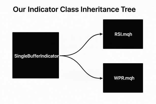
Fig. 1: Visualizing the inheritance tree of our family of single buffer indicators
To get the ball rolling, we will generalize the functionality we used when designing the RSI class so that it is appropriate for any indicator that has only 1 buffer. The reader should note that, MetaTrader 5 offers a comprehensive suite of indicators the reader can choose from. The fact that we are building a class for indicators with a single buffer, should inform the reader that there are indicators that have more than 1 buffer. When designing classes, generally we want the class to have a clear and definite purpose.
Trying to design a single class that handles all indicators, regardless of how many buffers they have, may prove too challenging to accomplish at once. Additionally, if you are not careful in your design, your code may contain logical errors and other unintentional bugs. Therefore, by limiting the scope of the class, we are setting ourselves up for success.
//+------------------------------------------------------------------+
//|                                        SingleBufferIndicator.mqh |
//|                                               Gamuchirai Ndawana |
//|                    https://www.mql5.com/en/users/gamuchiraindawa |
//+------------------------------------------------------------------+
#property copyright "Gamuchirai Ndawana"
#property link      "https://www.mql5.com/en/users/gamuchiraindawa"
#property version   "1.00"

class SingleBufferIndicator
  {

public:

   //--- Class methods
   bool              SetIndicatorValues(int buffer_size,bool set_as_series);
   double            GetReadingAt(int index);
   bool              SetDifferencedIndicatorValues(int buffer_size,int differencing_period,bool set_as_series);
   double            GetDifferencedReadingAt(int index);
   double            GetCurrentReading(void);

   //--- Have the indicator values been copied to the buffer?
   bool              indicator_values_initialized;
   bool              indicator_differenced_values_initialized;

   //--- How far into the future we wish to forecast
   int               forecast_horizon;

   //--- The buffer for our indicator
   double            indicator_reading[];
   vector            indicator_differenced_values;

   //--- The current size of the buffer the user last requested
   int               indicator_buffer_size;
   int               indicator_differenced_buffer_size;

   //--- The handler for our indicator
   int               indicator_handler;

   //--- The time frame our indicator should be applied on
   ENUM_TIMEFRAMES   indicator_time_frame;

   //--- The price should the indicator be applied on
   ENUM_APPLIED_PRICE indicator_price;

   //--- Give the user feedback
   string            user_feedback(int flag);

   //--- The Symbol our indicator should be applied on
   string            indicator_symbol;

   //--- Our period
   int               indicator_period;

   //--- Is our indicator valid?
   bool              IsValid(void);

   //---- Testing the Single Buffer Indicator Class
   //--- This method should be deleted in production
   virtual void      Test(void);
  };
//+------------------------------------------------------------------+
We now need a method that will copy the indicator readings from our indicator handler, to the indicator buffer. The method has 2 parameters, one specifying the amount of data to be copied, and the other specifies how we want to order the data. When the second parameter is true, the data is ordered from the past coming towards the present.
//+------------------------------------------------------------------+
//| Set our indicator values and our buffer size                     |
//+------------------------------------------------------------------+
bool              SingleBufferIndicator::SetIndicatorValues(int buffer_size,bool set_as_series)
  {

//--- Buffer size
   indicator_buffer_size = buffer_size;
   CopyBuffer(this.indicator_handler,0,0,buffer_size,indicator_reading);

//--- Should the array be set as series?
   if(set_as_series)
      ArraySetAsSeries(this.indicator_reading,true);
   indicator_values_initialized = true;

//--- Did something go wrong?
   vector indicator_test;
   indicator_test.CopyIndicatorBuffer(indicator_handler,0,0,buffer_size);
   if(indicator_test.Sum() == 0)
      return(false);

//--- Everything went fine.
   return(true);
  }
In machine learning, recording the change in a variable may be more informative than the raw reading. Therefore, let us also create a dedicated method that will calculate the change in the indicator's reading and copy it for us into an indicator buffer.
//+--------------------------------------------------------------+
//| Let's set the conditions for our differenced data            |
//+--------------------------------------------------------------+
bool              SingleBufferIndicator::SetDifferencedIndicatorValues(int buffer_size,int differencing_period,bool set_as_series)
  {
//--- Internal variables
   indicator_differenced_buffer_size = buffer_size;
   indicator_differenced_values = vector::Zeros(indicator_differenced_buffer_size);

//--- Prepare to record the differences in our RSI readings
   double temp_buffer[];
   int fetch = (indicator_differenced_buffer_size + (2 * differencing_period));
   CopyBuffer(indicator_handler,0,0,fetch,temp_buffer);
   if(set_as_series)
      ArraySetAsSeries(temp_buffer,true);

//--- Fill in our values iteratively
   for(int i = indicator_differenced_buffer_size;i > 1; i--)
     {
      indicator_differenced_values[i-1] = temp_buffer[i-1] - temp_buffer[i-1+differencing_period];
     }

//--- If the norm of a vector is 0, the vector is empty!
   if(indicator_differenced_values.Norm(VECTOR_NORM_P) != 0)
     {
      Print(user_feedback(2));
      indicator_differenced_values_initialized = true;
      return(true);
     }

   indicator_differenced_values_initialized = false;
   Print(user_feedback(3));
   return(false);
  }
Now that we have defined methods for copying indicator values into buffers, we need methods for retrieving the data in those buffers. Note that we could've easily just declared the indicator buffer as a public member of the class allowing us to quickly retrieve the values we want. The problem with that approach is that it defeats the purpose of building a class, which is having a uniform way of reading and writing to objects.
//--- Get a differenced value at a specific index
double            SingleBufferIndicator::GetDifferencedReadingAt(int index)
  {
//--- Make sure we're not trying to call values beyond our index
   if(index > indicator_differenced_buffer_size)
     {
      Print(user_feedback(4));
      return(-1e10);
     }

//--- Make sure our values have been set
   if(!indicator_differenced_values_initialized)
     {
      //--- The user is trying to use values before they were set in memory
      Print(user_feedback(1));
      return(-1e10);
     }

//--- Return the differenced value of our indicator at a specific index
   if((indicator_differenced_values_initialized) && (index < indicator_differenced_buffer_size))
      return(indicator_differenced_values[index]);

//--- Something went wrong.
   return(-1e10);
  }
The previous method returned the differenced indicator reading, it needs a counterpart method that will return actual indicator readings as they appear on the indicator.
//+------------------------------------------------------------------+
//| Get a reading at a specific index from our RSI buffer            |
//+------------------------------------------------------------------+
double            SingleBufferIndicator::GetReadingAt(int index)
  {
//--- Is the user trying to call indexes beyond the buffer?
   if(index > indicator_buffer_size)
     {
      Print(user_feedback(4));
      return(-1e10);
     }

//--- Get the reading at the specified index
   if((indicator_values_initialized) && (index < indicator_buffer_size))
      return(indicator_reading[index]);

//--- User is trying to get values that were not set prior
   else
     {
      Print(user_feedback(1));
      return(-1e10);
     }
  }
I also thought it would be useful to have a function dedicated for returning the indicator value at index 0, that is to say the current indicator reading.
//+------------------------------------------------------------------+
//| Get our current reading from the RSI indicator                   |
//+------------------------------------------------------------------+
double SingleBufferIndicator::GetCurrentReading(void)
  {
   double temp[];
   CopyBuffer(this.indicator_handler,0,0,1,temp);
   return(temp[0]);
  }
This function will inform us if our handler has been loaded correctly. It is a useful safety feature for us.
//+------------------------------------------------------------------+
//| Check if our indicator handler is valid                          |
//+------------------------------------------------------------------+
bool SingleBufferIndicator::IsValid(void)
  {
   return((this.indicator_handler != INVALID_HANDLE));
  }
As our user interacts with the indicator class, we want to give them prompts on any mistakes they may have made, and the appropriate solution to fix the error.
//+------------------------------------------------------------------+
//| Give the user feedback on the actions he is performing           |
//+------------------------------------------------------------------+
string SingleBufferIndicator::user_feedback(int flag)
  {
   string message;

//--- Check if the indicator loaded correctly
   if(flag == 0)
     {
      //--- Check the indicator was loaded correctly
      if(IsValid())
         message = "Indicator Class Loaded Correcrtly \nSymbol: " + (string) indicator_symbol + "\nPeriod: " + (string) indicator_period;
      return(message);
      //--- Something went wrong
      message = "Error loading Indicator: [ERROR] " + (string) GetLastError();
      return(message);
     }

//--- User tried getting indicator values before setting them
   if(flag == 1)
     {
      message = "Please set the indicator values before trying to fetch them from memory, call SetIndicatorValues()";
      return(message);
     }

//--- We sueccessfully set our differenced indicator values
   if(flag == 2)
     {
      message = "Succesfully set differenced indicator values.";
      return(message);
     }

//--- Failed  to set our differenced indicator values
   if(flag == 3)
     {
      message = "Failed to set our differenced indicator values: [ERROR] " + (string) GetLastError();
      return(message);
     }

//--- The user is trying to retrieve an index beyond the buffer size and must update the buffer size first
   if(flag == 4)
     {
      message = "The user is attempting to use call an index beyond the buffer size, update the buffer size first";
      return(message);
     }

//--- The class has been deactivated by the user
   if(flag == 5)
     {
      message = "Goodbye.";
      return(message);
     }

//--- No feedback
   else
      return("");
  }
With that done, we can now build our WPR class that will inherit from its parent the SingleBufferIndicator class. All in all, your dependency tree should resemble something like Fig 1 if you intend on following the article.
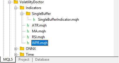
Fig. 2: Our dependency tree for our indicator classes
Let us now move on to the first step we will take in our WPR class, which will be including the SingleBufferIndicator class into the WPR class.
//+------------------------------------------------------------------+
//|                                                          WPR.mqh |
//|                                               Gamuchirai Ndawana |
//|                    https://www.mql5.com/en/users/gamuchiraindawa |
//+------------------------------------------------------------------+
#property copyright "Gamuchirai Ndawana"
#property link      "https://www.mql5.com/en/users/gamuchiraindawa"
#property version   "1.00"

//+------------------------------------------------------------------+
//| Load the parent class                                            |
//+------------------------------------------------------------------+
#include <VolatilityDoctor\Indicators\SingleBuffer\SingleBufferIndicator.mqh>
This time, before we define the class members of the WPR class, we will specify that the class extends the SingleBufferIndicator class by using the colon, ":", syntax. This is how we extend classes in MQL5. For readers unfamiliar with the concepts of OOP, extending a class allows us to call the methods we wrote in the SingleBufferIndicator class, from within the WPR class. By having our WPR and RSI class both extend the SingleBufferIndicator class, we will experience consistent functionality across both classes. Or in other words, all the public class members we built into our SingleBufferIndicator class will be readily available in any class that extends it.
//+------------------------------------------------------------------+
//| This class will provide us with usefull functionality for the WPR|
//+------------------------------------------------------------------+
class WPR : public SingleBufferIndicator
  {
public:
                     WPR();
                     WPR(string user_symbol,ENUM_TIMEFRAMES user_time_frame,int user_period);
                    ~WPR();
  };
The WPR and RSI indicators both have only 1 buffer; however, the indicators require different parameters to be initialized. Therefore, it makes more sense for the constructor to be specific to each indicator instance, since their constructor signatures can vary considerably from one indicator to the next.
//+------------------------------------------------------------------+
//| Our default constructor for our Indicator class                  |
//+------------------------------------------------------------------+
void WPR::WPR()
  {
   indicator_values_initialized       = false;
   indicator_symbol                   = "EURUSD";
   indicator_time_frame               = PERIOD_D1;
   indicator_period                   = 5;
   indicator_handler                  = iWPR(indicator_symbol,indicator_time_frame,indicator_period);
//--- Give the user feedback on initilization
   Print(user_feedback(0));
//--- Remind the user they called the default constructor
   Print("Default Constructor Called: ",__FUNCSIG__," ",&this);
  }
The parametric constructor allows the user to specify which symbol, time-frame and period the WPR indicator should be initialized with.
//+------------------------------------------------------------------+
//| Our parametric constructor for our Indicator class               |
//+------------------------------------------------------------------+
void WPR::WPR(string user_symbol,ENUM_TIMEFRAMES user_time_frame,int user_period)
  {
   indicator_values_initialized       = false;
   indicator_symbol                   = user_symbol;
   indicator_time_frame               = user_time_frame;
   indicator_period                   = user_period;
   indicator_handler                  = iWPR(indicator_symbol,indicator_time_frame,indicator_period);
//--- Give the user feedback on initilization
   Print(user_feedback(0));
  }
The class destructor will reset our important flags and release the indicator for us. It is good MQL5 practice to clean up after yourself, by building a dedicated class for this purpose, it reduces the cognitive load on the developer because you do not have to keep track of always, repeating the cleanup process when the class does it on your behalf.
//+------------------------------------------------------------------+
//| Our destructor for our Indicator class                           |
//+------------------------------------------------------------------+
void WPR::~WPR()
  {
//--- Free up resources we don't need and reset our flags
   if(IndicatorRelease(indicator_handler))
     {
      indicator_differenced_values_initialized = false;
      indicator_values_initialized = false;
      Print(user_feedback(5));
     }
  }
//+------------------------------------------------------------------+
Another functionality that we will need is the ability to identify when a new candle has been fully formed. Whenever this is the case, we would like to perform certain tasks. Therefore, we will dedicate a class for this objective since it is essential to us, and in some cases we may want to track the formation of candles on different timeframes at once. We will start off by declaring the class members needed by our Time class.
//+------------------------------------------------------------------+
//|                                                         Time.mqh |
//|                                               Gamuchirai Ndawana |
//|                    https://www.mql5.com/en/users/gamuchiraindawa |
//+------------------------------------------------------------------+
#property copyright "Gamuchirai Ndawana"
#property link      "https://www.mql5.com/en/users/gamuchiraindawa"
#property version   "1.00"

class Time
  {
private:
   datetime          time_stamp;
   datetime          current_time;
   string            selected_symbol;
   ENUM_TIMEFRAMES   selected_time_frame;
public:
                     Time(string user_symbol,ENUM_TIMEFRAMES user_time_frame);
   bool              NewCandle(void);
                    ~Time();
  };
Notice that the class does not have a default constructor, this has been done deliberately. Default constructors wouldn't make much sense in this particular case.
//+------------------------------------------------------------------+
//| Create our time object                                           |
//+------------------------------------------------------------------+
Time::Time(string user_symbol,ENUM_TIMEFRAMES user_time_frame)
  {
   selected_time_frame = user_time_frame;
   selected_symbol = user_symbol;
   current_time = iTime(user_symbol,selected_time_frame,0);
   time_stamp   = iTime(user_symbol,selected_time_frame,0);
  }
Currently, the class destructor is empty.
//+------------------------------------------------------------------+
//| Our destructor is currently empty                                |
//+------------------------------------------------------------------+
Time::~Time()
  {
  }
//+------------------------------------------------------------------+
Lastly, we need a method that will inform us if a new candle has been formed. This method will return true if a new candle has been formed, allowing us to perform our routines periodically.
//+------------------------------------------------------------------+
//| Check if a new candle has fully formed                           |
//+------------------------------------------------------------------+
bool Time::NewCandle(void)
  {
   current_time = iTime(selected_symbol,selected_time_frame,0);

//--- Check if a new candle has formed
   if(time_stamp != current_time)
     {
      time_stamp = current_time;
      return(true);
     }

//--- No new candle has completely formed
   return(false);
  }
Moving on, we will also need a dedicated class for handling our ONNX objects. As our projects grow bigger and more complicated, we do not want to repeat certain steps multiple times. Eventually, we may be better off having an ONNXFloat class for all our ONNX models that accept float data types. At the time of writing, the float data type is widely accepted as a stable data type to use when running ONNX models. Let us get started with the ONNX float class by defining its class members.
//+------------------------------------------------------------------+
//|                                                    ONNXFloat.mqh |
//|                                               Gamuchirai Ndawana |
//|                    https://www.mql5.com/en/users/gamuchiraindawa |
//+------------------------------------------------------------------+
#property copyright "Gamuchirai Ndawana"
#property link      "https://www.mql5.com/en/users/gamuchiraindawa"
#property version   "1.00"

//+------------------------------------------------------------------+
//| This class will help us work with ONNX Float models.             |
//+------------------------------------------------------------------+
class ONNXFloat
  {
private:
   //--- Our ONNX model handler
   long              onnx_model;
   int               onnx_outputs;
public:
   //--- Is our Model Valid?
   bool              OnnxModelIsValid(void);

   //--- Define the input shape of our model
   bool              DefineOnnxInputShape(int n_index,int n_stacks,int n_input_params);

   //--- Define the output shape of our model
   bool              DefineOnnxOutputShape(int n_index,int n_stacks, int n_output_params);

   vectorf           Predict(const vectorf &model_inputs);

   //--- ONNXFloat class constructor
                     ONNXFloat(const uchar &user_proto[]);

   //---- ONNXFloat class destructor
                    ~ONNXFloat();
  };
The constructor for our class accepts an ONNX model prototype and creates the ONNX model from the buffer passed by the user. Note that ONNX model buffers can only be passed by reference, not by value. The ampersand sign, "&", placed in front of the name of the ONNX model buffer "&user_proto" explicitly states that this parameter is a reference to an object in memory. Whenever a function has a parameter that is passed by reference, the user is expected to understand that any changes made to the parameter inside the function, will change the original parameter outside the function.
In our case, we do not intend to edit the ONNX prototype; therefore we modify the parameter to be "const" indicating to the programmer and to the compiler that no changes should be made. Therefore, if the programmer ignores our directives, the compiler will not accept that.
//+------------------------------------------------------------------+
//| Parametric Constructor For Our ONNXFloat class                   |
//+------------------------------------------------------------------+
ONNXFloat::ONNXFloat(const uchar &user_proto[])
  {
   onnx_model = OnnxCreateFromBuffer(user_proto,ONNX_DATA_TYPE_FLOAT);

   if(OnnxModelIsValid())
      Print("Volatility Doctor ONNXFloat Class Loaded Correctly: ",__FUNCSIG__," ",&this);

   else
      Print("Failed To Create The specified ONNX model: ",GetLastError());
  }
The ONNXFloat class destructor will release the memory that we assigned to our ONNX model automatically for us.
//+------------------------------------------------------------------+
//| Our ONNXFloat class destructor                                   |
//+------------------------------------------------------------------+
ONNXFloat::~ONNXFloat()
  {
   OnnxRelease(onnx_model);
  }
//+------------------------------------------------------------------+
We will also need a dedicated function that will inform us whether our ONNX model is valid by returning a Boolean flag that is only true if the model is valid.
//+------------------------------------------------------------------+
//| A method that returns true if our ONNXFloat model is valid       |
//+------------------------------------------------------------------+
bool ONNXFloat::OnnxModelIsValid(void)
  {
//--- Check if the model is valid
   if(onnx_model != INVALID_HANDLE)
      return(true);

//--- Something went wrong
   return(false);
  }
Setting up the input shape of any ONNX model is a necessary preparatory step that we will likely need frequently.
//+------------------------------------------------------------------+
//| Set the input shape of our ONNXFloat model                       |
//+------------------------------------------------------------------+
bool ONNXFloat::DefineOnnxInputShape(int n_index,int n_stacks,int n_input_params)
  {
   const ulong model_input_shape[] = {n_stacks,n_input_params};

   if(OnnxSetInputShape(onnx_model,n_index,model_input_shape))
     {
      Print("Succefully specified ONNX model output shape: ",__FUNCTION__," ",&this);
      return(true);
     }

//--- Something went wrong
   Print("Failed to set the passed ONNX model output shape: ",GetLastError());
   return(false);
  }
The same holds true for the ONNX model output shape.
//+------------------------------------------------------------------+
//| Set the output shape of our model                                |
//+------------------------------------------------------------------+
bool ONNXFloat::DefineOnnxOutputShape(int n_index,int n_stacks,int n_output_params)
  {
   const ulong model_output_shape[] = {n_output_params,n_stacks};
   onnx_outputs = n_output_params;

   if(OnnxSetOutputShape(onnx_model,n_index,model_output_shape))
     {
      Print("Succefully specified ONNX model input shape: ",__FUNCSIG__," ",&this);
      return(true);
     }

//--- Something went wrong
   Print("Failed to set the passed ONNX model input shape: ",GetLastError());
   return(false);
  }
Lastly, we need a predict function. This function will take the ONNX model's input data by reference, and since we do not intend on changing the input data, we modified that this parameter should be a constant. This prevents any unintentional side effects from corrupting the input data, most importantly, it instructs our compiler to prevent us from making any careless mistakes that would change the model inputs. Such safety features are invaluable, and having them built into your programming language qualifies MQL5 as a first-class Programming Language.
//+------------------------------------------------------------------+
//| Get a prediction from our model                                  |
//+------------------------------------------------------------------+
vectorf ONNXFloat::Predict(const vectorf &model_inputs)
  {
   vectorf model_output(onnx_outputs);
   if(OnnxRun(onnx_model,ONNX_DATA_TYPE_FLOAT,model_inputs,model_output))
     {
      vectorf res = model_output;
      return(res);
     }

   Comment("Failed to get a prediction from our ONNX model");
   Print("ONNX Run Failed: ",GetLastError());
   vectorf res = {10e8};
   return(res);
  }
The last class we will need is responsible for retrieving useful trade information for us, such as the minimum trade volume, or the current ask price.
//+------------------------------------------------------------------+
//|                                                    TradeInfo.mqh |
//|                                               Gamuchirai Ndawana |
//|                    https://www.mql5.com/en/users/gamuchiraindawa |
//+------------------------------------------------------------------+
#property copyright "Gamuchirai Ndawana"
#property link      "https://www.mql5.com/en/users/gamuchiraindawa"
#property version   "1.00"
class TradeInfo
  {
private:
                     string user_symbol;
                     ENUM_TIMEFRAMES user_time_frame;
                     double min_volume,max_volume,volume_step;
public:
                     TradeInfo(string selected_symbol,ENUM_TIMEFRAMES selected_time_frame);
                     double MinVolume(void);
                     double MaxVolume(void);
                     double VolumeStep(void);
                     double GetAsk(void);
                     double GetBid(void);
                     double GetClose(void);
                     string GetSymbol(void);
                    ~TradeInfo();
  };
The parametric class constructor takes 2 parameters specifying the intended symbol and time-frame.
//+------------------------------------------------------------------+
//| The constructor will load our symbol information                 |
//+------------------------------------------------------------------+
TradeInfo::TradeInfo(string selected_symbol,ENUM_TIMEFRAMES selected_time_frame)
  {
      //--- Which symbol are you interested in?
      user_symbol = selected_symbol;
      user_time_frame = selected_time_frame;

      if(SymbolSelect(user_symbol,true))
         {
            //--- Load symbol details
            min_volume = SymbolInfoDouble(user_symbol,SYMBOL_VOLUME_MIN);
            max_volume = SymbolInfoDouble(user_symbol,SYMBOL_VOLUME_MAX);
            volume_step = SymbolInfoDouble(user_symbol,SYMBOL_VOLUME_STEP);
            Print("Trade Info Loaded Successfully: ",__FUNCSIG__);
         }

      else
         {
            Print("Error Symbol Information Could Not Be Found For: ",selected_symbol," ",GetLastError());
         }

  }
We will also define methods for getting the current readings of each of the 4 primary price feeds, that is to say each of these methods returns the current Open, High, Low and Close prices respectively.
//+------------------------------------------------------------------+
//| Return the close of the selected symbol                          |
//+------------------------------------------------------------------+
double TradeInfo::GetClose(void)
   {
      double res = iClose(user_symbol,user_time_frame,0);
      return(res);
   }

//+------------------------------------------------------------------+
//| Return the open of the selected symbol                          |
//+------------------------------------------------------------------+
double TradeInfo::GetOpen(void)
   {
      double res = iOpen(user_symbol,user_time_frame,0);
      return(res);
   }

//+------------------------------------------------------------------+
//| Return the high of the selected symbol                          |
//+------------------------------------------------------------------+
double TradeInfo::GetHigh(void)
   {
      double res = iHigh(user_symbol,user_time_frame,0);
      return(res);
   }

//+------------------------------------------------------------------+
//| Return the low of the selected symbol                          |
//+------------------------------------------------------------------+
double TradeInfo::GetLow(void)
   {
      double res = iLow(user_symbol,user_time_frame,0);
      return(res);
   }
When working with multiple symbols, it is helpful to have a reminder of which symbol the current instance of the class has been assigned to.
//+------------------------------------------------------------------+
//| Return the selected symbol                                       |
//+------------------------------------------------------------------+
string TradeInfo::GetSymbol(void)
   {
      string res = user_symbol;
      return(res);
   }
Our class also provides wrappers to quickly retrieve important information regarding the permitted volume levels on the current symbol.
//+------------------------------------------------------------------+
//| Return the volume step allowed                                   |
//+------------------------------------------------------------------+
double TradeInfo::VolumeStep(void)
   {
      double res = volume_step;
      return(res);
   }

//+------------------------------------------------------------------+
//| Return the minimum volume allowed                                |
//+------------------------------------------------------------------+
double TradeInfo::MinVolume(void)
   {
      double res = min_volume;
      return(res);
   }

//+------------------------------------------------------------------+
//| Return the maximum volume allowed                                |
//+------------------------------------------------------------------+
double TradeInfo::MaxVolume(void)
   {
      double res = max_volume;
      return(res);
   }
We will also need the class to readily provide us with the current bid and ask prices.
//+------------------------------------------------------------------+
//| Return the current ask                                           |
//+------------------------------------------------------------------+
double TradeInfo::GetAsk(void)
   {
      return(SymbolInfoDouble(GetSymbol(),SYMBOL_ASK));
   }

//+------------------------------------------------------------------+
//| Return the current bid                                           |
//+------------------------------------------------------------------+
double TradeInfo::GetBid(void)
   {
      return(SymbolInfoDouble(GetSymbol(),SYMBOL_BID));
   }
Currently, our Time class destructor is empty.
//+------------------------------------------------------------------+
//| Destructor is currently empty                                    |
//+------------------------------------------------------------------+
TradeInfo::~TradeInfo()
  {
  }
//+------------------------------------------------------------------+
All in all, if you have been following along with us, then your tree of dependencies should resemble Fig 3 below.
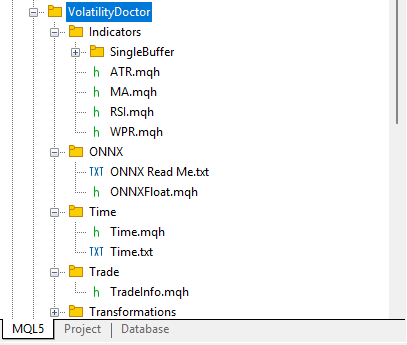
Fig. 3: These classes should be kept in a dependency tree that resembles ours, for readers following along
Now let us define the script that will fetch the relevant market data that we need. We want to first fetch the four primary price feeds (OHLC), followed by the growth in these 4 price feeds, and finally, we will write out the indicator data from our 14 WPR indicators.
//+------------------------------------------------------------------+
//|                                                      ProjectName |
//|                                      Copyright 2020, CompanyName |
//|                                       http://www.companyname.net |
//+------------------------------------------------------------------+
#property copyright "Copyright 2024, MetaQuotes Ltd."
#property link      "https://www.mql5.com"
#property version   "1.00"
#property script_show_inputs

//+------------------------------------------------------------------+
//| System constants                                                 |
//+------------------------------------------------------------------+
#define HORIZON 10

//+------------------------------------------------------------------+
//| Libraries                                                        |
//+------------------------------------------------------------------+
#include <VolatilityDoctor\Indicators\WPR.mqh>

//+------------------------------------------------------------------+
//| Global variables                                                 |
//+------------------------------------------------------------------+
WPR *my_wpr_array[14];
string file_name = Symbol() + " WPR Algorithmic Input Selection.csv";

//+------------------------------------------------------------------+
//| Inputs                                                           |
//+------------------------------------------------------------------+
input int size = 3000;

//+------------------------------------------------------------------+
//| Our script execution                                             |
//+------------------------------------------------------------------+
void OnStart()
  {
//--- How much data should we store in our indicator buffer?
   int fetch = size + (2 * HORIZON);

//--- Store pointers to our WPR objects
   for(int i = 0; i <= 13; i++)
     {
      //--- Create an WPR object
      my_wpr_array[i] = new WPR(Symbol(),PERIOD_CURRENT,((i+1) * 5));
      //--- Set the WPR buffers
      my_wpr_array[i].SetIndicatorValues(fetch,true);
      my_wpr_array[i].SetDifferencedIndicatorValues(fetch,HORIZON,true);
     }

//---Write to file
   int file_handle=FileOpen(file_name,FILE_WRITE|FILE_ANSI|FILE_CSV,",");

   for(int i=size;i>=1;i--)
     {
      if(i == size)
        {
         FileWrite(file_handle,"Time","True Open","True High","True Low","True Close","Open","High","Low","Close","WPR 5","WPR 10","WPR 15","WPR 20","WPR 25","WPR 30","WPR 35","WPR 40","WPR 45","WPR 50","WPR 55","WPR 60","WPR 65","WPR 70","Diff WPR 5","Diff WPR 10","Diff WPR 15","Diff WPR 20","Diff WPR 25","Diff WPR 30","Diff WPR 35","Diff WPR 40","Diff WPR 45","Diff WPR 50","Diff WPR 55","Diff WPR 60","Diff WPR 65","Diff WPR 70");
        }

      else
        {
         FileWrite(file_handle,
                   iTime(_Symbol,PERIOD_CURRENT,i),
                   iOpen(_Symbol,PERIOD_CURRENT,i),
                   iHigh(_Symbol,PERIOD_CURRENT,i),
                   iLow(_Symbol,PERIOD_CURRENT,i),
                   iClose(_Symbol,PERIOD_CURRENT,i),
                   iOpen(_Symbol,PERIOD_CURRENT,i) - iOpen(Symbol(),PERIOD_CURRENT,i + HORIZON),
                   iHigh(_Symbol,PERIOD_CURRENT,i) - iHigh(Symbol(),PERIOD_CURRENT,i + HORIZON),
                   iLow(_Symbol,PERIOD_CURRENT,i) - iLow(Symbol(),PERIOD_CURRENT,i + HORIZON),
                   iClose(_Symbol,PERIOD_CURRENT,i) - iClose(Symbol(),PERIOD_CURRENT,i + HORIZON),
                   my_wpr_array[0].GetReadingAt(i),
                   my_wpr_array[1].GetReadingAt(i),
                   my_wpr_array[2].GetReadingAt(i),
                   my_wpr_array[3].GetReadingAt(i),
                   my_wpr_array[4].GetReadingAt(i),
                   my_wpr_array[5].GetReadingAt(i),
                   my_wpr_array[6].GetReadingAt(i),
                   my_wpr_array[7].GetReadingAt(i),
                   my_wpr_array[8].GetReadingAt(i),
                   my_wpr_array[9].GetReadingAt(i),
                   my_wpr_array[10].GetReadingAt(i),
                   my_wpr_array[11].GetReadingAt(i),
                   my_wpr_array[12].GetReadingAt(i),
                   my_wpr_array[13].GetReadingAt(i),
                   my_wpr_array[0].GetDifferencedReadingAt(i),
                   my_wpr_array[1].GetDifferencedReadingAt(i),
                   my_wpr_array[2].GetDifferencedReadingAt(i),
                   my_wpr_array[3].GetDifferencedReadingAt(i),
                   my_wpr_array[4].GetDifferencedReadingAt(i),
                   my_wpr_array[5].GetDifferencedReadingAt(i),
                   my_wpr_array[6].GetDifferencedReadingAt(i),
                   my_wpr_array[7].GetDifferencedReadingAt(i),
                   my_wpr_array[8].GetDifferencedReadingAt(i),
                   my_wpr_array[9].GetDifferencedReadingAt(i),
                   my_wpr_array[10].GetDifferencedReadingAt(i),
                   my_wpr_array[11].GetDifferencedReadingAt(i),
                   my_wpr_array[12].GetDifferencedReadingAt(i),
                   my_wpr_array[13].GetDifferencedReadingAt(i)
                  );
        }
     }
//--- Close the file
   FileClose(file_handle);

//--- Delete our WPR object pointers
   for(int i = 0; i <= 13; i++)
     {
      delete my_wpr_array[i];
     }
  }
//+------------------------------------------------------------------+
#undef HORIZON
Analyzing Our Data With Python
Once you have finished, apply the script to your chosen market so that we will have market data to analyze. We are applying the script to the EURGBP pair in this discussion, and now that our data is ready, let us load our Python libraries for analysis.
#Load the libraries
import pandas as pd
import numpy as np
import seaborn as sns
import matplotlib.pyplot as plt
Read in the data.
#Read in the data
data = pd.read_csv("..\EURGBP WPR Algorithmic Input Selection.csv")

#Label the data
HORIZON = 10
data['Target'] = data['Close'].shift(-HORIZON) - data['Close']

#Drop the last 10 rows
data = data.iloc[:-HORIZON,:]
Create copies of the input and target.
#Define inputs and target
X = data.iloc[:,1:-1].copy()
y = data.iloc[:,-1].copy()
Scale and center each numerical column in the dataset.
#Store Z-scores
Z1 = X.mean()
Z2 = X.std()

#Scale the data
X = ((X - Z1)/ Z2)
Load the numerical libraries we need to test our accuracy.
from sklearn.model_selection import cross_val_score,TimeSeriesSplit
from sklearn.linear_model import Ridge
Create a time-series cross validation object.
tscv = TimeSeriesSplit(n_splits=5,gap=HORIZON)sdvdsvds Define a method that will always return our cross-validated accuracy levels.
#Return our cross validated accuracy
def score(f_model,f_X,f_y):
    return(np.mean(np.abs(cross_val_score(f_model,f_X,f_y,scoring='neg_mean_squared_error',cv=tscv,n_jobs=-1))))
We will also need a dedicated method to return a new model, this ensures that we aren't leaking data to the models we use.
def get_model():
    return(Ridge())
Keeping a column entirely full of zeros allows you to measure the accuracy of always predicting the average market return.
X['Null'] = 0
Record the error produced by always predicting the average market return(total sum of squares/TSS). Now that we have recorded the error threshold defined by always predicting the average market return, we can now confidently assert that any model that produces error levels greater than 0.000324 has no skill that impresses us, as far as this discussion is concerned.
#This will be the last entry in our list of results
#Record our error if we always predict the average market return (total sum of squares/TSS)
tss = score(get_model(),X[['Null']],y)
tss
0.00032439931180771236
We will now create an array to help us keep track of our results.
res = []
The first result we want to record, is our error levels using OHLC market data in its original form.
#This will be our first entry in our list of results
#Record our error using OHLC price data
res.append(score(get_model(),X.iloc[:,:8],y))
Next, we would like to know our error levels only using the 14 WPR indicator periods we selected.
#Second
#Record our error using just indicators
res.append(score(get_model(),X.iloc[:,8:-1],y))
Finally, let us record our error levels using all the data we have available.
#Third
#Record our error using all the data we have
res.append(score(get_model(),X.iloc[:,:-1],y))
Now load the UMAP library. Our original data has 36 columns, the UMAP library will help us represent this data using any number of columns greater than or equal to 1 and less than the original number of columns. This new representation of the data, may be more informative than the data was in its original form. Hence, in this sense, Dimension Reduction algorithms can also be thought of as a family of methods that allow us to effectively use all the data we have describing our problem.
import umap
We want to search for a number of embeddings that are at most 2 less the original number of columns.
EPOCHS = X.iloc[:,:-1].shape[1] - 2
Iteratively embed the data using UMAP. The number of embedded columns to be produced will be increased from 1, in increments of 1 step, until the upper bound we set in the previous line of code.
for i in range(EPOCHS):
    reducer = umap.UMAP(n_components=(i+1),metric='euclidean',random_state=0,transform_seed=0,n_neighbors=30)
    X_embedded = pd.DataFrame(reducer.fit_transform(X.iloc[:,:-1]))
    res.append(score(get_model(),X_embedded,y))
Join our results.
res.append(tss)
The red solid line is our critical error benchmark, the error produced by always predicting the average market return (TSS). The red dotted line is the lowest error level we managed to produce. This corresponds to the model that was built when our original data was embedded into 2 columns by our UMAP algorithm. Notice that, this error level outperforms the TSS by a wider margin than what we were able to achieve when using the market data in its original form. We are essentially using all the WPR periods at once, in a manner that is more meaningful than what we could've achieved otherwise.
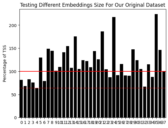
Fig. 4: Using 2 embedded UMAP components, we outperformed an equivalent model using all the market data in its original form
Transform the data using the ideal UMAP settings we identified.
reducer = umap.UMAP(n_components=2,metric='euclidean',random_state=0,transform_seed=0,n_neighbors=30)
X_embedded = pd.DataFrame(reducer.fit_transform(X.iloc[:,:-1]))
Label our 2 classes. This will help us later to visualize what UMAP is doing to our data.
data['Class'] = 0

data.loc[data['Target'] > 0,'Class'] = 1
Prepare a dataset to store the transformed data.
umap_data =pd.DataFrame(columns=['UMAP 1','UMAP 2'])
Store the embedded price levels.
umap_data['UMAP 1'] = X_embedded.iloc[:,0]
umap_data['UMAP 2'] = X_embedded.iloc[:,1]
Without UMAP, our data is challenging to visualize meaningfully due to the high number of dimensions. In fact, the best we can do is create pairs of scatter plots; otherwise, there is no way of effectively visualizing 36 dimensions at once. In Fig 5 and 6 below, the red dots indicate bullish price action and black represents bearish price action.
fig , axs = plt.subplots(2,2)

fig.suptitle('Visualizing EURGBP 2002-2025 Daily Price Data')

axs[0,0].scatter(data.loc[data['Target']>0 ,'Open'],data.loc[data['Target']>0 ,'Close'],color='red')
axs[0,0].scatter(data.loc[data['Target']<0 ,'Open'],data.loc[data['Target']<0 ,'Close'],color='black')

axs[0,1].scatter(data.loc[data['Target']>0 ,'True Open'],data.loc[data['Target']>0 ,'True Close'],color='red')
axs[0,1].scatter(data.loc[data['Target']<0 ,'True Open'],data.loc[data['Target']<0 ,'True Close'],color='black')

axs[1,1].scatter(data.loc[data['Target']>0 ,'WPR 5'],data.loc[data['Target']>0 ,'WPR 50'],color='red')
axs[1,1].scatter(data.loc[data['Target']<0 ,'WPR 5'],data.loc[data['Target']<0 ,'WPR 50'],color='black')

axs[1,0].scatter(data.loc[data['Target']>0 ,'WPR 15'],data.loc[data['Target']>0 ,'WPR 25'],color='red')
axs[1,0].scatter(data.loc[data['Target']<0 ,'WPR 15'],data.loc[data['Target']<0 ,'WPR 25'],color='black')
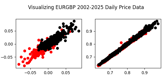
Fig 5: On the left we have plotted the change in open price against the change in close price. While on the right, we have plotted the true open and close price.
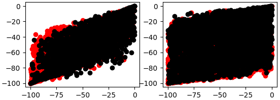
Fig. 6:The left scatter plot is expressing the relationship between the 5 and 50 period WPR, while the right is the 15 and 25 period WPR
As we can see, Fig 5 and Fig 6 are challenging to interpret meaningfully, there are no clear patterns in the data. Additionally, it can be dangerous to create 2-dimensional scatter plots of phenomena happening in more than 2 dimensions. This is because, what appears to be a relationship between the 2 variables may be explained by other dimensions we cannot include in one plot. This may lead us to false discoveries or unreasonable confidence in relationships that aren't as stable as they appear.
However, after applying UMAP, we can easily plot all the data we have, in just 2 dimensions. We can generally see that low and high values of the first embedding appear to be associated with bearish and bullish price action, respectively.
sns.scatterplot(x=X_embedded.iloc[:,0],y=X_embedded.iloc[:,1],hue=data['Class'])
plt.grid()
plt.ylabel('Second UMAP Embedding')
plt.xlabel('First UMAP Embedding')
plt.title('Visualizing The Most Effective Embedding We Found')
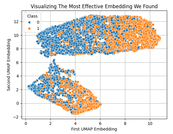
Fig. 7: Visualizing our UMAP embeddings of the original market data
Let us now get ready to prepare our models for back-testing. Import the library we need.
from sklearn.model_selection import train_test_split
Split the market data. Our training samples run from November 2002 until August 2018, so our back test period will start in September 2018.
train , test = train_test_split(data,test_size=0.3,shuffle=False)
train
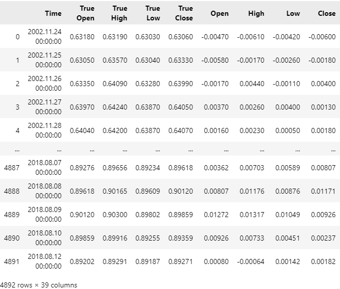
Fig. 8: Viewing our market data in its original form
Let us now load in our statistical model.
from sklearn.neural_network import MLPRegressor
Scale the train data.
#Sample mean
Z1 = train.iloc[:,1:-2].mean()

#Sample standard deviation
Z2 = train.iloc[:,1:-2].std()

train_scaled = train.copy()

train_scaled.iloc[:,1:-2] = ((train.iloc[:,1:-2] - Z1) / Z2)
Embed the training data.
reducer = umap.UMAP(n_components=2,metric='euclidean',random_state=0,transform_seed=0,n_neighbors=30)
X_embedded = pd.DataFrame(reducer.fit_transform(train_scaled.iloc[:,1:-2],columns=['UMAP 1','UMAP 2']))
Our framework follows a 2-step process. First, fit a model that learns to approximate the UMAP algorithm. This substitutes the need of rewriting the UMAP algorithm from scratch in MQL5. The UMAP algorithm is fairly sophisticated, and was implemented by a team of Post Doctoral Researchers. It takes considerable effort for researchers to write a numerically stable implementation of an algorithm. Therefore, it is not generally considered sound practice to try and implement such algorithms on your own.
#Learn To Estimate UMAP Embeddings From The Data
umap_model = MLPRegressor(shuffle=False,hidden_layer_sizes=(train.iloc[:,1:-2].shape[1],10,20,100,20,10,2),random_state=0,solver='lbfgs',activation='relu',learning_rate='constant',learning_rate_init=1e-4,power_t=1e-1)
np.mean(np.abs(cross_val_score(umap_model,train.iloc[:,1:-2],X_embedded,scoring='neg_mean_squared_error',n_jobs=-1)))
11.2489992665160363
Learn the UMAP function.
umap_model.fit(train.iloc[:,1:-2],X_embedded)
predictions = umap_model.predict(train.iloc[:,1:-2])
Now we need a model that forecasts the EURGBP market return, given the UMAP embeddings of the market. In scikit-learn our neural network models have an important parameter named, "random_state". This parameter affects the initial weights and biases that the neural network starts with. Depending on the problem at hand, training the model multiple times with different initial states, can lead to considerable variation in performance levels, as we can see in Fig 9 below.
EPOCHS = 100
res = []

for i in range(EPOCHS):
    #Try different random states
    model = MLPRegressor(shuffle=False,early_stopping=False,hidden_layer_sizes=(2,1,10,20,1),activation='identity',solver='lbfgs',random_state=i,max_iter=int(2e5))
    res.append(score(model,predictions,train['Target']))
Visualizing our results.
plt.plot(res,color='black')
plt.axhline(np.min(res),color='red',linestyle=':')
plt.scatter(res.index(np.min(res)),np.min(res),color='red')
plt.grid()
plt.ylabel('Cross Validated RMSE')
plt.xlabel('Neural Network Random State')
plt.title('Our Neural Network Performance With Different Initial Conditions')
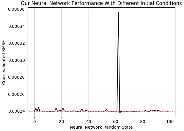
Fig. 9: Visualizing the optimal initial state for our neural network in this problem
Our chosen neural network is predicting the 10-Day EURGBP market return with 38% less error than always predicting the average market return.
tss = score(Ridge(),train[['Close']]*0,train['Target'])
1-(np.min(res)/tss)
0.3822093585025088
Fit the model using the optimal random state we identified in Fig 9.
embedded_model = MLPRegressor(shuffle=False,early_stopping=False,hidden_layer_sizes=(2,1,10,20,1),activation='identity',solver='lbfgs',random_state=res.index(np.min(res)),max_iter=int(2e5))
embedded_model.fit(predictions,train['Target'])
Load the libraries we need to convert the model to ONNX format.
import onnx
from skl2onnx import convert_sklearn
from skl2onnx.common.data_types import FloatTensorType
Define the parameter shapes of our models.
umap_model_input_shape = [("float_input",FloatTensorType([1,train.iloc[:,1:-2].shape[1]]))]
umap_model_output_shape = [("float_output",FloatTensorType([X_embedded.iloc[:,:].shape[1],1]))]

embedded_model_input_shape = [("float_input",FloatTensorType([1,X_embedded.iloc[:,:].shape[1]]))]
embedded_model_output_shape = [("float_output",FloatTensorType([1,1]))]
Convert the ONNX models into their prototypes.
umap_proto = convert_sklearn(umap_model,initial_types=umap_model_input_shape,final_types=umap_model_output_shape,target_opset=12)
embeded_proto = convert_sklearn(embedded_model,initial_types=embedded_model_input_shape,final_types=embedded_model_output_shape,target_opset=12)
Save the prototypes to disk.
onnx.save(umap_proto,"EURGBP WPR Ridge UMAP.onnx")
onnx.save(embeded_proto,"EURGBP WPR Ridge EMBEDDED.onnx")
Building Our Application in MQL5
Now let us start building our application. We will first need to specify system constants that aren't going to change in our program.
//+------------------------------------------------------------------+
//|                             EURGBP Multiple Periods Analysis.mq5 |
//|                                               Gamuchirai Ndawana |
//|                    https://www.mql5.com/en/users/gamuchiraindawa |
//+------------------------------------------------------------------+
#property copyright "Gamuchirai Ndawana"
#property link      "https://www.mql5.com/en/users/gamuchiraindawa"
#property version   "1.00"

//+------------------------------------------------------------------+
//| REMINDER:                                                        |
//| These ONNX models were trained with Daily EURGBP data ranging    |
//| from 24 November 2002 until 12 August 2018. Test the strategy    |
//| outside of these time periods, on the Daily Time-Frame for       |
//| reliable results.                                                |
//+------------------------------------------------------------------+

//+------------------------------------------------------------------+
//| System definitions                                               |
//+------------------------------------------------------------------+

//--- ONNX Model I/O Parameters
#define UMAP_INPUTS 36
#define UMAP_OUTPUTS 2
#define EMBEDDED_INPUTS  2
#define EMBEDDED_OUTPUTS 1

//--- Our forecasting periods
#define HORIZON 10

//--- Our desired time frame
#define SYSTEM_TIMEFRAME_1 PERIOD_D1
Now, let us load our ONNX models.
//+------------------------------------------------------------------+
//| Load our ONNX models as resources                                |
//+------------------------------------------------------------------+

//--- ONNX Model Prototypes
#resource  "\\Files\\EURGBP WPR UMAP.onnx" as const uchar umap_proto[];
#resource  "\\Files\\EURGBP WPR EMBEDDED.onnx" as const uchar embedded_proto[];
Then, we will load the libraries we need for our application.
//+------------------------------------------------------------------+
//| Libraries We Need                                                |
//+------------------------------------------------------------------+
#include <Trade\Trade.mqh>
#include <VolatilityDoctor\Time\Time.mqh>
#include <VolatilityDoctor\Indicators\WPR.mqh>
#include <VolatilityDoctor\ONNX\OnnxFloat.mqh>
#include <VolatilityDoctor\Trade\TradeInfo.mqh>
Define the global variables we will use throughout our program. Notice that we must define just a handful of global variables, this is what we meant in the introduction of our discussion when we said that OOP helps us control the namespace of our applications. Most of the variables and objects we are using have been neatly packed away inside the classes we wrote.
//+------------------------------------------------------------------+
//| Global varaibles                                                 |
//+------------------------------------------------------------------+
CTrade Trade;
TradeInfo *TradeInformation;

//--- Our time object let's us know when a new candle has fully formed on the specified time-frame
Time *eurgbp_daily;

//--- All our different William's Percent Range Periods will be kept in a single array
WPR *wpr_array[14];

//--- Our ONNX class objects have usefull functions designed for rapid ONNX development
ONNXFloat *umap_onnx,*embedded_onnx;

//--- Model forecast
double expected_return;

int position_timer;
We also copied over the Z1 and Z2 scores we used to scale our training data in Python.
//--- The average column values from the training set
double Z1[] = {7.84311120e-01,  7.87104135e-01,  7.81713516e-01,  7.84343731e-01,
               5.23887980e-04,  5.26022077e-04,  5.25382257e-04,  5.25688880e-04,
               -5.08398234e+01, -5.07130228e+01, -5.05834313e+01, -5.04425081e+01,
               -5.02709031e+01, -5.01349627e+01, -5.00653250e+01, -5.01661938e+01,
               -5.03082375e+01, -5.04550339e+01, -5.05861939e+01, -5.06434696e+01,
               -5.07286211e+01, -5.07819768e+01,  1.96979782e-02,  5.29204133e-02,
               4.12732506e-02,  3.20037455e-02,  2.61762719e-02,  2.34184127e-02,
               2.62342592e-02,  3.32894491e-02,  3.81853070e-02,  3.85464026e-02,
               3.85499926e-02,  3.94004124e-02,  4.02388908e-02,  4.02388908e-02
               };

//--- The column standard deviation from the training set
double Z2[] = {8.29473604e-02, 8.35406090e-02, 8.23981331e-02, 8.28950223e-02,
               1.21995172e-02, 1.22880295e-02, 1.20471133e-02, 1.21798952e-02,
               3.00742110e+01, 3.05948913e+01, 3.05244154e+01, 3.03776475e+01,
               3.02862706e+01, 3.00844693e+01, 2.98788650e+01, 2.97182936e+01,
               2.95133008e+01, 2.93983475e+01, 2.92679071e+01, 2.91072869e+01,
               2.90154368e+01, 2.89821474e+01, 4.32293242e+01, 4.43537714e+01,
               4.02730688e+01, 3.66106699e+01, 3.41930128e+01, 3.21743917e+01,
               3.03647897e+01, 2.87462989e+01, 2.73771066e+01, 2.63857585e+01,
               2.54625376e+01, 2.43656339e+01, 2.33983568e+01, 2.26334633e+01
              };
Upon initialization, we will set up our indicators and initialize our custom classes. If our classes fail to load correctly, then we will break the initialization procedure and give the user feedback on what went wrong.
//+------------------------------------------------------------------+
//| Expert initialization function                                   |
//+------------------------------------------------------------------+
int OnInit()
  {
//--- Do no display the indicators, they will clutter our view
   TesterHideIndicators(true);

//--- Setup our pointers to our WPR objects
   update_indicators();

//--- Get trade information on the symbol
   TradeInformation = new TradeInfo(Symbol(),SYSTEM_TIMEFRAME_1);

//--- Create our ONNXFloat objects
   umap_onnx     = new ONNXFloat(umap_proto);
   embedded_onnx = new ONNXFloat(embedded_proto);

//--- Create our Time management object
   eurgbp_daily = new Time(Symbol(),SYSTEM_TIMEFRAME_1);

//--- Check if the models are valid
   if(!umap_onnx.OnnxModelIsValid())
      return(INIT_FAILED);
   if(!embedded_onnx.OnnxModelIsValid())
      return(INIT_FAILED);

//--- Reset our position timer
   position_timer = 0;

//--- Specify the models I/O shapes
   if(!umap_onnx.DefineOnnxInputShape(0,1,UMAP_INPUTS))
      return(INIT_FAILED);
   if(!embedded_onnx.DefineOnnxInputShape(0,1,EMBEDDED_INPUTS))
      return(INIT_FAILED);

   if(!umap_onnx.DefineOnnxOutputShape(0,1,UMAP_OUTPUTS))
      return(INIT_FAILED);
   if(!embedded_onnx.DefineOnnxOutputShape(0,1,EMBEDDED_OUTPUTS))
      return(INIT_FAILED);

//---
   return(INIT_SUCCEEDED);
  }
Upon deinitialization, we will clean up after ourselves and delete the pointers we created for our objects. This is good programming practice in MQL5 and prevents problems such as memory leakage or buffer overflows if we have multiple instances of this application running on one machine but none of them clean up after themselves. Also, an important note, developers with experience outside MQL5, especially from languages such as C, may be already familiar with pointers as a memory-address.
An important distinction needs to be made here; The safety features embedded in MQL5 do not permit direct access to memory. Rather, the clever developers from the MetaQuotes team found a workaround solution that creates a unique identifier for each object, and then they intelligently bound each unique identifier with its associated object. Therefore, readers that are already familiar with pointers from their independent studies should note that the MQL5 implementation of a pointer does not literally give the developer any memory addresses because the developers of MQL5 viewed that as a security vulnerability.
//+------------------------------------------------------------------+
//| Expert deinitialization function                                 |
//+------------------------------------------------------------------+
void OnDeinit(const int reason)
  {
//--- Delete the pointers for our custom objects
   delete umap_onnx;
   delete embedded_onnx;
   delete eurgbp_daily;
   //--- Delete all pointers to our WPR objects
   for(int i = 0; i <= 13; i++)
     {
         delete wpr_array[i];
     }
  }
Every time we receive updated prices, we will call the Time class to check if a new daily candle has been formed, if this is the case, we will update our indicator readings and then subsequently search for a trading opportunity if we have no open trades, or manage any trades we have opened.
//+------------------------------------------------------------------+
//| Expert tick function                                             |
//+------------------------------------------------------------------+
void OnTick()
  {
//--- Do we have a new daily candle?
   if(eurgbp_daily.NewCandle())
     {
      static int i = 0;
      Print(i+=1);
      update_indicators();

      if(PositionsTotal() == 0)
        {
         position_timer =0;
         find_setup();
        }

      else
         if((PositionsTotal() > 0) && (position_timer < HORIZON))
            position_timer += 1;

         else
            if((PositionsTotal() > 0) && (position_timer >= (HORIZON -1)))
               Trade.PositionClose(Symbol());

      Comment("Position Timer: ",position_timer);
     }
  }
Find a trading setup simply requires that we fetch the relevant market data and prepare it as our ONNX model inputs. Note that we subtract the mean of each column and divide by the column standard deviation before we finally store the input data into a constant vectorf type. We then pass this constant vector to our ONNXFloat.Predict() method and obtain a forecast from our model. Building these classes has helped us reduce the total number of lines of code we need to write, by a considerable factor.
//+------------------------------------------------------------------+
//| Find A Trading Setup For Us                                      |
//+------------------------------------------------------------------+
void find_setup(void)
  {
//--- Update our indicators
   update_indicators();

//--- Prepare our input vector
   vectorf market_state(UMAP_INPUTS);

//--- Fill in the Market Data that has to embedded into UMAP form
   market_state[0] = (float) iOpen(_Symbol,SYSTEM_TIMEFRAME_1,0);
   market_state[1] = (float) iHigh(_Symbol,SYSTEM_TIMEFRAME_1,0);
   market_state[2] = (float) iLow(_Symbol,SYSTEM_TIMEFRAME_1,0);
   market_state[3] = (float) iClose(_Symbol,SYSTEM_TIMEFRAME_1,0);
   market_state[4] = (float)(iOpen(_Symbol,SYSTEM_TIMEFRAME_1,0) - iOpen(Symbol(),SYSTEM_TIMEFRAME_1,HORIZON));
   market_state[5] = (float)(iHigh(_Symbol,SYSTEM_TIMEFRAME_1,0) - iHigh(Symbol(),SYSTEM_TIMEFRAME_1,HORIZON));
   market_state[6] = (float)(iLow(_Symbol,SYSTEM_TIMEFRAME_1,0) - iLow(Symbol(),SYSTEM_TIMEFRAME_1,HORIZON));
   market_state[7] = (float)(iClose(_Symbol,SYSTEM_TIMEFRAME_1,0) - iClose(Symbol(),SYSTEM_TIMEFRAME_1,HORIZON));
   market_state[8] = (float) wpr_array[0].GetReadingAt(0);
   market_state[9] = (float) wpr_array[1].GetReadingAt(0);
   market_state[10] = (float) wpr_array[2].GetReadingAt(0);
   market_state[11] = (float) wpr_array[3].GetReadingAt(0);
   market_state[12] = (float) wpr_array[4].GetReadingAt(0);
   market_state[13] = (float) wpr_array[5].GetReadingAt(0);
   market_state[14] = (float) wpr_array[6].GetReadingAt(0);
   market_state[15] = (float) wpr_array[7].GetReadingAt(0);
   market_state[16] = (float) wpr_array[8].GetReadingAt(0);
   market_state[17] = (float) wpr_array[9].GetReadingAt(0);
   market_state[18] = (float) wpr_array[10].GetReadingAt(0);
   market_state[19] = (float) wpr_array[11].GetReadingAt(0);
   market_state[20] = (float) wpr_array[12].GetReadingAt(0);
   market_state[21] = (float) wpr_array[13].GetReadingAt(0);
   market_state[22] = (float) wpr_array[0].GetDifferencedReadingAt(0);
   market_state[23] = (float) wpr_array[1].GetDifferencedReadingAt(0);
   market_state[24] = (float) wpr_array[2].GetDifferencedReadingAt(0);
   market_state[25] = (float) wpr_array[3].GetDifferencedReadingAt(0);
   market_state[26] = (float) wpr_array[4].GetDifferencedReadingAt(0);
   market_state[27] = (float) wpr_array[5].GetDifferencedReadingAt(0);
   market_state[27] = (float) wpr_array[6].GetDifferencedReadingAt(0);
   market_state[29] = (float) wpr_array[7].GetDifferencedReadingAt(0);
   market_state[30] = (float) wpr_array[8].GetDifferencedReadingAt(0);
   market_state[31] = (float) wpr_array[9].GetDifferencedReadingAt(0);
   market_state[32] = (float) wpr_array[10].GetDifferencedReadingAt(0);
   market_state[33] = (float) wpr_array[11].GetDifferencedReadingAt(0);
   market_state[34] = (float) wpr_array[12].GetDifferencedReadingAt(0);
   market_state[35] = (float) wpr_array[13].GetDifferencedReadingAt(0);

//--- Standardize and scale each input
   for(int i =0; i < UMAP_INPUTS;i++)
     {
      market_state[i] = (float)((market_state[i] - Z1[i]) / Z2[i]);
     };

   const vectorf onnx_inputs = market_state;

   const vectorf umap_predictions = umap_onnx.Predict(onnx_inputs);
   Print("UMAP Model Returned Embeddings: ",umap_predictions);

   const vectorf expected_eurgbp_return = embedded_onnx.Predict(umap_predictions);
   Print("Embeddings Model Expects EURGBP Returns: ",expected_eurgbp_return);
   expected_return = expected_eurgbp_return[0];

   vector o,c;

   o.CopyRates(Symbol(),SYSTEM_TIMEFRAME_1,COPY_RATES_OPEN,0,HORIZON);
   c.CopyRates(Symbol(),SYSTEM_TIMEFRAME_1,COPY_RATES_CLOSE,0,HORIZON);

   bool bullish_reversal   = o.Mean() < c.Mean();
   bool bearish_reversal   = o.Mean() > c.Mean();

   if(bearish_reversal)
     {
      if(expected_return > 0)
        {
         Trade.Buy((TradeInformation.MinVolume()*2),Symbol(),TradeInformation.GetAsk(),0,0,"");
         return;
        }

      Trade.Buy(TradeInformation.MinVolume(),Symbol(),TradeInformation.GetAsk(),0,0,"");
      return;
     }

   else
      if(bullish_reversal)
        {
         if(expected_return < 0)
           {
            Trade.Sell((TradeInformation.MinVolume()*2),Symbol(),TradeInformation.GetBid(),0,0,"");
           }

         Trade.Sell(TradeInformation.MinVolume(),Symbol(),TradeInformation.GetBid(),0,0,"");
         return;
        }

  }
This is the implementation of the method we call to update our technical indicators.
//+------------------------------------------------------------------+
//| Update our indicator readings                                    |
//+------------------------------------------------------------------+
void update_indicators(void)
  {
//--- Store pointers to our WPR objects
   for(int i = 0; i <= 13; i++)
     {
      //--- Create an WPR object
      wpr_array[i] = new WPR(Symbol(),SYSTEM_TIMEFRAME_1,((i+1) * 5));
      //--- Set the WPR buffers
      wpr_array[i].SetIndicatorValues(60,true);
      wpr_array[i].SetDifferencedIndicatorValues(60,HORIZON,true);
     }
  }
Finally, always remember to undefine system constants you built, at the end of your program.
//+------------------------------------------------------------------+
//| Undefine system constants we no longer need                      |
//+------------------------------------------------------------------+
#undef EMBEDDED_INPUTS
#undef EMBEDDED_OUTPUTS
#undef UMAP_INPUTS
#undef UMAP_OUTPUTS
#undef HORIZON
#undef SYSTEM_TIMEFRAME_1
//+------------------------------------------------------------------+
When you launch your application, it should look something like Fig 10 below. This is expected, and all we need to do is write one more line of code into our initialization procedure that instructs our terminal not to display indicators during testing.
//--- Do no display the indicators, they will clutter our view
   TesterHideIndicators(true);
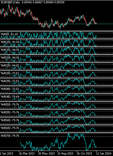
Fig. 10: Our view will initially be cluttered, due to the high number of indicators we are using
Once that is done, we can begin our back test. Recall that our training samples ran from November 2002 until August 2018; therefore our back test period should've started in September 2018, until the present day. Unfortunately, my internet connection was not reliable, and I was unable to safely download the historical data from my broker. Therefore, I had to instead perform the test from the beginning of 2023 until the present day.
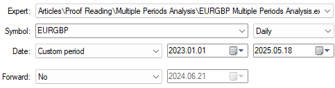
Fig. 11: The dates for our back-test period
We always prefer using all ticks based on real-ticks to get a realistic emulation of past market performance. This can be demanding on your network because the volume of data requested will be large.
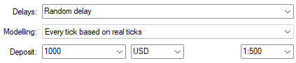
Fig. 12: The settings which we used for our back-test are also important
The classes we built will give you constant feedback during back-testing. We can check for any errors by reading the printed messages. As we can see in Fig 13, our classes are running as expected without any error messages being logged.
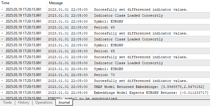
Fig. 13: The classes we built will give you feedback during back-testing. The feedback should be positive and always end with the model forecast if you have no open positions
We can also visualize the equity curve produced by our strategy. The equity curve has a positive long-term uptrend, which encourages us to continue developing the strategy and look for more safety features to limit the losses if possible.
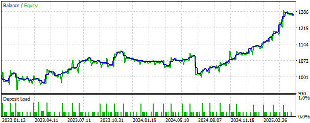
Fig. 14: Visualizing the equity curve produced by our trading strategy
Finally, we can also visualize a detailed analysis of the performance of our trading strategy. As we can see, our strategy had an accuracy level of 58% from all the trades it placed, with a Sharpe ratio of 0.90.
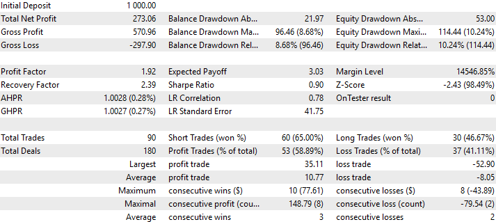
Fig. 15: A detailed analysis of the performance of our trading strategy on data it has not seen before
Conclusion
Through this discussion, the reader walks away with actionable insights on the practical benefits of statistical modelling, beyond the ordinary task of price prediction. We illustrated to the reader that:
- Machine learning can be used for money management: By increasing our lot size when our model aligned with our trading signal, we are effectively giving the statistical model control over the trading volume, allowing our computer to place bigger trades when it is "feeling confident".
- Machine learning can also be used to uncover more meaningful ways of looking at data: We can use a family of machine learning algorithms known as dimension reduction methods, to compact our data, allowing use to expose the important patterns in large datasets.
This means that, the reader can substitute the WPR indicator, with a combination of their favorite indicators, and by applying dimension reduction techniques as demonstrated in this article, you may find novel representations of your private strategies that may improve your trading performance, as we saw earlier when we outperformed all the market data we had on hand, using a UMAP representation of only 2 columns from the original 36 columns.
The reader additionally receives many benefits from using the UMAP algorithm suggested in this article, over popular choices such as PCA (Principal Components Analysis). We will highlight a few material benefits:
- UMAP is a non-linear method: Popular dimension reduction techniques such as PCA inherently assume that there exists a linear relationship in the data. The algorithms fail when this assumption is not true. UMAP, on the other hand, is explicitly intended to look for non-linear relationships. The reader should not say that UMAP is more "powerful" than PCA, but rather it is more appropriate to say that UMAP is more "flexible" than PCA.
- UMAP is Geometric And Not Euclidean: This to say, UMAP sees shapes, not just straight line distances. Unlike methods like PCA that slice data with straight lines, UMAP bends with your data. It doesn’t assume the world is flat, rather, it assumes your data lives on a curved surface called a Riemannian manifold, a concept from the mathematical study of topology that helps describe complex, nonlinear spaces. This lets UMAP preserve the true geometry of your data, not by flattening it, but rather by flowing with it.
Lastly, the reader has benefited from an appreciation of the value of Object-Oriented Programming in MQL5. While OOP may be considered an old technology, it still holds immense value by allowing us to centralize control and all failures to a single file. It saves us time from having to repeat boilerplate code, allowing us to rapidly execute our ideas with predictable outcomes.
| File Name | File Description |
|---|---|
| Use_All_Data.ipynb | The Jupyter Notebook we used to analyze our market data. |
| Fetch_Data_Algorithmic_Input_Selection.mq5 | The MQL5 script we used to fetch the market data we needed. |
| EURGBP_Multiple_Periods_Analysis.mq5 | The Expert Advisor we built together that used 14 different WPR periods, at once. |
| EURGBP_WPR_Algorithmic_Input_Selection.csv | The historical market data we fetched from our broker. |
| EURGBP_WPR_EMBEDDED.onnx | The ONNX model responsible for approximating our 36 columns of data, down to 2 UMAP embeddings. |
| EURGBP_WPR_UMAP.onnx | The ONNX model responsible for forecasting the EURGBP market return, given 2 UMAP embeddings. |
| EURGBP_Multiple_Periods_Analysis.ex5 | A compiled version of our Expert Advisor. |
Warning: All rights to these materials are reserved by MetaQuotes Ltd. Copying or reprinting of these materials in whole or in part is prohibited.
This article was written by a user of the site and reflects their personal views. MetaQuotes Ltd is not responsible for the accuracy of the information presented, nor for any consequences resulting from the use of the solutions, strategies or recommendations described.

- Free trading apps
- Over 8,000 signals for copying
- Economic news for exploring financial markets
You agree to website policy and terms of use