Chaos theory in trading (Part 2): Diving deeper

Previous article summary

The first article considered basic concepts of chaos theory and their application to the analysis of financial markets. We looked at key concepts, such as attractors, fractals, and the butterfly effect, and discussed how they reveal themselves in market dynamics. Particular attention was paid to the characteristics of chaotic systems in the context of finance and the concept of volatility.

We also compared classical chaos theory with Bill Williams' approach, which allowed us to better understand the differences between the scientific and practical application of these concepts in trading. Lyapunov exponent as a tool for analyzing financial time series took a central stage in the article. We considered both its theoretical meaning and a practical implementation of its calculation in MQL5 language.

The final part of the article was devoted to the statistical analysis of trend reversals and continuations using the Lyapunov exponent. Using the EURUSD pair on H1 timeframe as an example, we demonstrated how this analysis can be applied in practice and discussed the interpretation of the results obtained.

The article laid the foundation for understanding chaos theory in the context of financial markets and presented practical tools for applying it to trading. In the second article, we will continue to deepen our understanding of this topic, focusing on more complex aspects and their practical applications.

The first thing we will talk about is fractal dimension as a measure of market chaos.

Fractal dimension as a measure of market chaos

Fractal dimension is a concept that plays an important role in chaos theory and the analysis of complex systems, including financial markets. It provides a quantitative measure of the complexity and self-similarity of an object or process, making it particularly useful for assessing the degree of randomness in market movements.

In the context of financial markets, fractal dimension can be used to measure the "jaggedness" of price charts. A higher fractal dimension indicates a more complex, chaotic price structure, while a lower dimension may indicate smoother, predictable movement.

There are several methods for calculating fractal dimension. One of the most popular ones is the box-counting method. This method involves covering the chart with a grid of cells of varying sizes and counting the number of cells needed to cover the chart at different scales.

The equation for calculating the fractal dimension D using the method is as follows:

D = -lim(ε→0) [log N(ε) / log(ε)]

where N(ε) is the number of cells of size ε required to cover the object.

Applying fractal dimension to financial market analysis can provide traders and analysts with additional insight into the nature of market movements. For example:

• Identifying market modes: Changes in fractal dimension can indicate transitions between different market states such as trends, flat movements, or chaotic periods.
• Volatility assessment: High fractal dimension often corresponds to periods of increased volatility.
• Forecasting: Analyzing changes in fractal dimension over time can help in forecasting future market movements.
• Optimizing trading strategies: Understanding the fractal structure of the market can help in developing and optimizing trading algorithms.

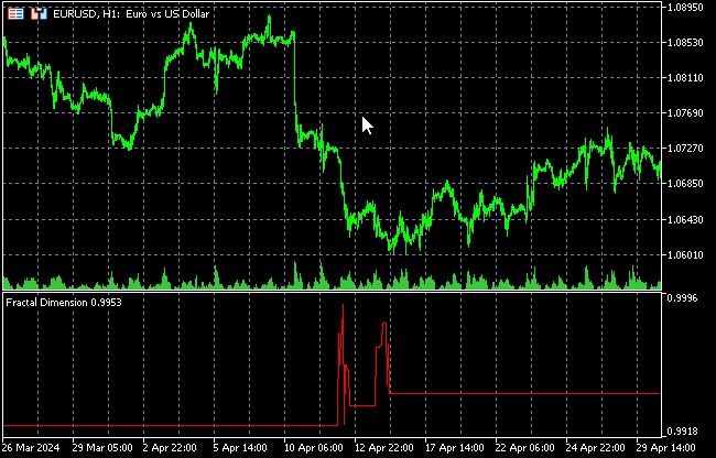
Now let's look at the practical implementation of calculating the fractal dimension in the MQL5 language. We will develop an indicator that will calculate the fractal dimension of the price chart in real time in MQL5.

The indicator uses the box-counting method to estimate the fractal dimension.

#property copyright "Copyright 2024, Evgeniy Shtenco"
#property link      "https://www.mql5.com/en/users/koshtenko"
#property version   "1.00"
#property strict
#property indicator_separate_window
#property indicator_buffers 1
#property indicator_plots   1
#property indicator_label1  "Fractal Dimension"
#property indicator_type1   DRAW_LINE
#property indicator_color1  clrRed
#property indicator_style1  STYLE_SOLID
#property indicator_width1  1

input int    InpBoxSizesCount = 5;    // Number of box sizes
input int    InpMinBoxSize    = 2;    // Minimum box size
input int    InpMaxBoxSize    = 100;  // Maximum box size
input int    InpDataLength    = 1000; // Data length for calculation

double FractalDimensionBuffer[];

int OnInit()
{
   SetIndexBuffer(0, FractalDimensionBuffer, INDICATOR_DATA);
   IndicatorSetInteger(INDICATOR_DIGITS, 4);
   IndicatorSetString(INDICATOR_SHORTNAME, "Fractal Dimension");
   return(INIT_SUCCEEDED);
}

int OnCalculate(const int rates_total,
                const int prev_calculated,
                const datetime &time[],
                const double &open[],
                const double &high[],
                const double &low[],
                const double &close[],
                const long &tick_volume[],
                const long &volume[],
                const int &spread[])
{
   int start;
   if(prev_calculated == 0)
      start = InpDataLength;
   else
      start = prev_calculated - 1;
   
   for(int i = start; i < rates_total; i++)
   {
      FractalDimensionBuffer[i] = CalculateFractalDimension(close, i);
   }
   
   return(rates_total);
}

double CalculateFractalDimension(const double &price[], int index)
{
   if(index < InpDataLength)
      return 0;
   
   double x[]; 
   double y[];
   ArrayResize(x, InpBoxSizesCount);
   ArrayResize(y, InpBoxSizesCount);
   
   for(int i = 0; i < InpBoxSizesCount; i++)
   {
      int boxSize = (int)MathRound(MathPow(10, MathLog10(InpMinBoxSize) + (MathLog10(InpMaxBoxSize) - MathLog10(InpMinBoxSize)) * i / (InpBoxSizesCount - 1)));
      x[i] = MathLog(1.0 / boxSize);
      y[i] = MathLog(CountBoxes(price, index, boxSize));
   }
   
   double a, b;
   CalculateLinearRegression(x, y, InpBoxSizesCount, a, b);
   
   return a; // The slope of the regression line is the estimate of the fractal dimension
}

int CountBoxes(const double &price[], int index, int boxSize)
{
   double min = price[index - InpDataLength];
   double max = min;
   
   for(int i = index - InpDataLength + 1; i <= index; i++)
   {
      if(price[i] < min) min = price[i];
      if(price[i] > max) max = price[i];
   }
   
   return (int)MathCeil((max - min) / (boxSize * _Point));
}

void CalculateLinearRegression(const double &x[], const double &y[], int count, double &a, double &b)
{
   double sumX = 0, sumY = 0, sumXY = 0, sumX2 = 0;
   
   for(int i = 0; i < count; i++)
   {
      sumX += x[i];
      sumY += y[i];
      sumXY += x[i] * y[i];
      sumX2 += x[i] * x[i];
   }
   
   a = (count * sumXY - sumX * sumY) / (count * sumX2 - sumX * sumX);
   b = (sumY - a * sumX) / count;
}

The indicator calculates the fractal dimension of a price chart using the box-counting method. Fractal dimension is a measure of the "jaggedness" or complexity of a chart and can be used to assess the degree of chaos in the market.

Inputs:

• InpBoxSizesCount - number of different "box" sizes for calculation
• InpMinBoxSize - minimum "box" size
• InpMaxBoxSize - maximum "box" size
• InpDataLength - number of candles used for calculation

Indicator operation algorithm:

1. For each point on the chart, the indicator calculates the fractal dimension using data for the last InpDataLength candles.
2. The box-counting method is applied with different "box" sizes from InpMinBoxSize to InpMaxBoxSize.
3. The number of "boxes" required to cover the chart is calculated for each "box" size.
4. A dependence graph of the logarithm of the number of "boxes" on the logarithm of the size of the "box" is created.
5. The graph slope is calculated using the linear regression method, which is an estimate of the fractal dimension.

Changes in fractal dimension may signal a change in the market mode.

Recurrence analysis to uncover hidden patterns in price movements

Recurrence analysis is a powerful method of non-linear time series analysis that can be effectively applied to study the dynamics of financial markets. This approach allows us to visualize and quantify recurring patterns in complex dynamic systems, which certainly include financial markets.

The main tool of recurrence analysis is the recurrence plot. This diagram is a visual representation of the repeating states of a system over time. In a recurrence diagram, a point (i, j) is colored if the states at times i and j are similar in a certain sense.

To construct a recurrence diagram of a financial time series, follow these steps:

1. Phase space reconstruction: Using the delay method, we transform the one-dimensional price time series into a multidimensional phase space.
2. Determining the similarity threshold: We select a criterion, by which we will consider two states to be similar.
3. Construction of the recurrence matrix: For each pair of time points, we determine whether the corresponding states are similar.
4. Visualization: We display the recurrence matrix as a two-dimensional image, where similar states are indicated by dots.

Recurrence diagrams allow us to identify different types of dynamics in a system:

• Homogeneous regions indicate stationary periods
• Diagonal lines indicate deterministic dynamics
• Vertical and horizontal structures may indicate laminar conditions
• The absence of a structure is characteristic of a random process.

To quantify the structures in a recurrence diagram, various recurrence measures are used, such as the percentage of recurrence, the entropy of diagonal lines, the maximum length of a diagonal line, and others.

Applying recurrence analysis to financial time series can help:

1. Identify different market modes (trend, flat, chaotic state)
2. Detect mode change
3. Assess the predictability of the market in different periods
4. Reveal hidden cyclical patterns

For practical implementation of recurrent analysis in trading, we can develop an indicator in the MQL5 language, which will build a recurrence diagram and calculate recurrence measures in real time. Such an indicator can serve as an additional tool for making trading decisions, especially when combined with other technical analysis methods.

In the next section, we will look at a specific implementation of such an indicator and discuss how to interpret its readings in the context of a trading strategy.

Recurrence analysis indicator in MQL5

The indicator implements the recurrence analysis method for studying the dynamics of financial markets. It calculates three key measures of recurrence: recurrence level, determinism and laminarity.

#property copyright "Copyright 2024, Evgeniy Shtenco"
#property link      "https://www.mql5.com/en/users/koshtenko"
#property version   "1.00"
#property strict
#property indicator_separate_window
#property indicator_buffers 3
#property indicator_plots   3
#property indicator_label1  "Recurrence Rate"
#property indicator_type1   DRAW_LINE
#property indicator_color1  clrBlue
#property indicator_label2  "Determinism"
#property indicator_type2   DRAW_LINE
#property indicator_color2  clrRed
#property indicator_label3  "Laminarity"
#property indicator_type3   DRAW_LINE
#property indicator_color3  clrGreen

input int    InpEmbeddingDimension = 3;     // Embedding dimension
input int    InpTimeDelay          = 1;     // Time delay
input int    InpThreshold          = 10;    // Threshold (in points)
input int    InpWindowSize         = 200;   // Window size

double RecurrenceRateBuffer[];
double DeterminismBuffer[];
double LaminarityBuffer[];

int minRequiredBars;

int OnInit()
{
   SetIndexBuffer(0, RecurrenceRateBuffer, INDICATOR_DATA);
   SetIndexBuffer(1, DeterminismBuffer, INDICATOR_DATA);
   SetIndexBuffer(2, LaminarityBuffer, INDICATOR_DATA);
   
   IndicatorSetInteger(INDICATOR_DIGITS, 4);
   IndicatorSetString(INDICATOR_SHORTNAME, "Recurrence Analysis");
   
   minRequiredBars = InpWindowSize + (InpEmbeddingDimension - 1) * InpTimeDelay;
   
   return(INIT_SUCCEEDED);
}

int OnCalculate(const int rates_total,
                const int prev_calculated,
                const datetime &time[],
                const double &open[],
                const double &high[],
                const double &low[],
                const double &close[],
                const long &tick_volume[],
                const long &volume[],
                const int &spread[])
{
   if(rates_total < minRequiredBars) return(0);
   
   int start = (prev_calculated > 0) ? MathMax(prev_calculated - 1, minRequiredBars - 1) : minRequiredBars - 1;
   
   for(int i = start; i < rates_total; i++)
   {
      CalculateRecurrenceMeasures(close, rates_total, i, RecurrenceRateBuffer[i], DeterminismBuffer[i], LaminarityBuffer[i]);
   }
   
   return(rates_total);
}

void CalculateRecurrenceMeasures(const double &price[], int price_total, int index, double &recurrenceRate, double &determinism, double &laminarity)
{
   if(index < minRequiredBars - 1 || index >= price_total)
   {
      recurrenceRate = 0;
      determinism = 0;
      laminarity = 0;
      return;
   }

   int windowStart = index - InpWindowSize + 1;
   int matrixSize = InpWindowSize - (InpEmbeddingDimension - 1) * InpTimeDelay;
   
   int recurrenceCount = 0;
   int diagonalLines = 0;
   int verticalLines = 0;
   
   for(int i = 0; i < matrixSize; i++)
   {
      for(int j = 0; j < matrixSize; j++)
      {
         bool isRecurrent = IsRecurrent(price, price_total, windowStart + i, windowStart + j);
         if(isRecurrent)
         {
            recurrenceCount++;
            
            // Check for diagonal lines
            if(i > 0 && j > 0 && IsRecurrent(price, price_total, windowStart + i - 1, windowStart + j - 1))
               diagonalLines++;
            
            // Check for vertical lines
            if(i > 0 && IsRecurrent(price, price_total, windowStart + i - 1, windowStart + j))
               verticalLines++;
         }
      }
   }
   
   recurrenceRate = (double)recurrenceCount / (matrixSize * matrixSize);
   determinism = (recurrenceCount > 0) ? (double)diagonalLines / recurrenceCount : 0;
   laminarity = (recurrenceCount > 0) ? (double)verticalLines / recurrenceCount : 0;
}

bool IsRecurrent(const double &price[], int price_total, int i, int j)
{
   if(i < 0 || j < 0 || i >= price_total || j >= price_total) return false;

   double distance = 0;
   for(int d = 0; d < InpEmbeddingDimension; d++)
   {
      int offset = d * InpTimeDelay;
      if(i + offset >= price_total || j + offset >= price_total) return false;
      double diff = price[i + offset] - price[j + offset];
      distance += diff * diff;
   }
   distance = MathSqrt(distance);
   
   return (distance <= InpThreshold * _Point);
}

Main characteristics of the indicator:

The indicator is displayed in a separate window below the price chart and uses three buffers to store and display data. The indicator calculates three metrics: Recurrence Rate (blue line), which shows the overall level of recurrence, Determinism (red line), which is a measure of the system predictability, and Laminarity (green line), which evaluates the tendency of the system to remain in a certain state.

The indicator inputs include InpEmbeddingDimension (default 3), which defines the embedding dimension for the phase space reconstruction, InpTimeDelay (default 1) for the time delay during reconstruction, InpThreshold (default 10) for the state similarity threshold in points, and InpWindowSize (default 200) for setting the size of the analysis window.

The indicator operating algorithm is based on the delay method for reconstructing the phase space from a one-dimensional time series of prices. For each point in the analysis window, its "recurrence" in relation to other points is calculated. Then, based on the obtained recurrent structure, three measures are calculated: Recurrence Rate, which determines the proportion of recurrence points in the total number of points, Determinism, which shows the proportion of recurrence points that form diagonal lines, and Laminarity, which estimates the proportion of recurrence points that form vertical lines.

Applying Takens' embedding theorem in volatility forecasting

Takens' embedding theorem is a fundamental result in the theory of dynamical systems that has important implications for the analysis of time series, including financial data. This theorem states that a dynamic system can be reconstructed from observations of just one variable using the time-lag method.

In the context of financial markets, Takens' theorem allows us to reconstruct a multidimensional phase space from a one-dimensional time series of prices or returns. This is particularly useful when analyzing volatility, which is a key characteristic of financial markets.

The basic steps in applying Takens' theorem to forecast volatility are:

1. Phase space reconstruction:
   • Selecting the embedding dimension (m)
   • Selecting the time delay (τ)
   • Creating m-dimensional vectors from the original time series
2. Analysis of the reconstructed space:
   • Finding the nearest neighbors for each point
   • Estimation of local point density
3. Volatility forecast:
   • Using local density information to estimate future volatility

Let's look at these steps in more detail.

Phase space reconstruction:

Let us have a time series of close prices {p(t)}. We create m-dimensional vectors as follows:

x(t) = [p(t), p(t+τ), p(t+2τ), ..., p(t+(m-1)τ)]

where m is an embedding dimension and τ is a time delay.

Choosing the correct values of m and τ is critical for successful reconstruction. Typically, τ is chosen using mutual information or auto correlation function methods, and m is chosen using the false nearest neighbor method.

Analysis of the reconstructed space:

After reconstructing the phase space, we can analyze the structure of the system attractor. For volatility forecasting, information about the local density of points in phase space is especially important.

For each point x(t), we find its k nearest neighbors (usually k is chosen in the range from 5 to 20) and calculate the average distance to these neighbors. This distance serves as a measure of local density and hence local volatility.

Volatility forecast

The basic idea of forecasting volatility using reconstructed phase space is that points close in this space are likely to have similar behavior in the near future.

To forecast volatility at t+h time point, we:

• Find the k nearest neighbors for the current x(t) point in the reconstructed space
• Calculate the actual volatility for these neighbors h steps ahead
• Use the average of these volatilities as a forecast

Mathematically this can be expressed as follows:

σ̂(t+h) = (1/k) Σ σ(ti+h), where ti are the indices of the k nearest neighbors of x(t)

The advantages of this approach:

• It takes into account non-linear market dynamics
• It does not require assumptions about the distribution of returns
• We are able to pick up complex patterns in volatility

Cons:

• It is sensitive to the choice of parameters (m, τ, k)
• It can be computationally expensive for large amounts of data

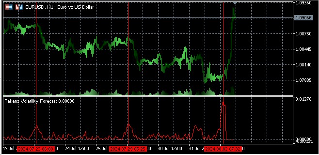
Implementation

Let's create an MQL5 indicator that will implement this volatility forecast method:

#property copyright "Copyright 2024, Evgeniy Shtenco"
#property link      "https://www.mql5.com/en/users/koshtenko"
#property version   "1.00"
#property strict
#property indicator_separate_window
#property indicator_buffers 1
#property indicator_plots   1
#property indicator_label1  "Predicted Volatility"
#property indicator_type1   DRAW_LINE
#property indicator_color1  clrRed
#property indicator_style1  STYLE_SOLID
#property indicator_width1  1

input int    InpEmbeddingDimension = 3;     // Embedding dimension
input int    InpTimeDelay          = 5;     // Time delay
input int    InpNeighbors          = 10;    // Number of neighbors
input int    InpForecastHorizon    = 10;    // Forecast horizon
input int    InpLookback           = 1000;  // Lookback period

double PredictedVolatilityBuffer[];

int OnInit()
{
   SetIndexBuffer(0, PredictedVolatilityBuffer, INDICATOR_DATA);
   IndicatorSetInteger(INDICATOR_DIGITS, 5);
   IndicatorSetString(INDICATOR_SHORTNAME, "Takens Volatility Forecast");
   return(INIT_SUCCEEDED);
}

int OnCalculate(const int rates_total,
                const int prev_calculated,
                const datetime &time[],
                const double &open[],
                const double &high[],
                const double &low[],
                const double &close[],
                const long &tick_volume[],
                const long &volume[],
                const int &spread[])
{
   int start = MathMax(prev_calculated, InpLookback + InpEmbeddingDimension * InpTimeDelay + InpForecastHorizon);
   
   for(int i = start; i < rates_total; i++)
   {
      if (i >= InpEmbeddingDimension * InpTimeDelay && i + InpForecastHorizon < rates_total)
      {
         PredictedVolatilityBuffer[i] = PredictVolatility(close, i);
      }
   }
   
   return(rates_total);
}

double PredictVolatility(const double &price[], int index)
{
   int vectorSize = InpEmbeddingDimension;
   int dataSize = InpLookback;
   
   double currentVector[];
   ArrayResize(currentVector, vectorSize);
   for(int i = 0; i < vectorSize; i++)
   {
      int priceIndex = index - i * InpTimeDelay;
      if (priceIndex < 0) return 0;  // Prevent getting out of array
      currentVector[i] = price[priceIndex];
   }
   
   double distances[];
   ArrayResize(distances, dataSize);
   
   for(int i = 0; i < dataSize; i++)
   {
      double sum = 0;
      for(int j = 0; j < vectorSize; j++)
      {
         int priceIndex = index - i - j * InpTimeDelay;
         if (priceIndex < 0) return 0;  // Prevent getting out of array
         double diff = currentVector[j] - price[priceIndex];
         sum += diff * diff;
      }
      distances[i] = sqrt(sum);
   }
   
   int sortedIndices[];
   ArrayCopy(sortedIndices, distances);
   ArraySort(sortedIndices);
   
   double sumVolatility = 0;
   for(int i = 0; i < InpNeighbors; i++)
   {
      int neighborIndex = index - sortedIndices[i];
      if (neighborIndex + InpForecastHorizon >= ArraySize(price)) return 0;  // Prevent getting out of array
      double futureReturn = (price[neighborIndex + InpForecastHorizon] - price[neighborIndex]) / price[neighborIndex];
      sumVolatility += MathAbs(futureReturn);
   }
   
   return sumVolatility / InpNeighbors;
}

Methods for determining a time delay and an embedding dimension

When reconstructing the phase space using Takens' theorem, it is critical to choose two key parameters correctly: the time delay (τ) and the embedding dimension (m). Incorrect selection of these parameters can lead to incorrect reconstruction and, as a consequence, to erroneous conclusions. Let's consider two main methods for determining these parameters.

Autocorrelation function (ACF) method for determining time delay

The method is based on the idea of choosing a time delay τ, at which the autocorrelation function first crosses zero or reaches a certain low value, for example, 1/e of the initial value. This allows one to choose a delay, at which successive values of the time series become sufficiently independent of each other.

The implementation of the ACF method in MQL5 may look like this:

int FindOptimalLagACF(const double &price[], int maxLag, double threshold = 0.1)
{
   int size = ArraySize(price);
   if(size <= maxLag) return 1;
   
   double mean = 0;
   for(int i = 0; i < size; i++)
      mean += price[i];
   mean /= size;
   
   double variance = 0;
   for(int i = 0; i < size; i++)
      variance += MathPow(price[i] - mean, 2);
   variance /= size;
   
   for(int lag = 1; lag <= maxLag; lag++)
   {
      double acf = 0;
      for(int i = 0; i < size - lag; i++)
         acf += (price[i] - mean) * (price[i + lag] - mean);
      acf /= (size - lag) * variance;
      
      if(MathAbs(acf) <= threshold)
         return lag;
   }
   
   return maxLag;
}

In this implementation, we first calculate the mean and variance of the time series. Then, for each lag from 1 to maxLag, we calculate the value of the autocorrelation function. Once the ACF value becomes less than or equal to a given threshold (default 0.1), we return this lag as the optimal time delay.

ACF method has its pros and cons. On the one hand, it is easy to implement and intuitive. On the other hand, it does not take into account non-linear dependencies in the data, which can be a significant drawback when analyzing financial time series, which often exhibit non-linear behavior.

Mutual information (MI) method for determining time delay

This method is based on information theory and is able to take into account non-linear dependencies in data. The idea is to choose a delay τ that corresponds to the first local minimum of the mutual information function.

The implementation of the mutual information method in MQL5 may look like this:

double CalculateMutualInformation(const double &price[], int lag, int bins = 20)
{
   int size = ArraySize(price);
   if(size <= lag) return 0;
   
   double minPrice = price[ArrayMinimum(price)];
   double maxPrice = price[ArrayMaximum(price)];
   double binSize = (maxPrice - minPrice) / bins;
   
   int histogram[];
   ArrayResize(histogram, bins * bins);
   ArrayInitialize(histogram, 0);
   
   int totalPoints = 0;
   
   for(int i = 0; i < size - lag; i++)
   {
      int bin1 = (int)((price[i] - minPrice) / binSize);
      int bin2 = (int)((price[i + lag] - minPrice) / binSize);
      if(bin1 >= 0 && bin1 < bins && bin2 >= 0 && bin2 < bins)
      {
         histogram[bin1 * bins + bin2]++;
         totalPoints++;
      }
   }
   
   double mutualInfo = 0;
   for(int i = 0; i < bins; i++)
   {
      for(int j = 0; j < bins; j++)
      {
         if(histogram[i * bins + j] > 0)
         {
            double pxy = (double)histogram[i * bins + j] / totalPoints;
            double px = 0, py = 0;
            for(int k = 0; k < bins; k++)
            {
               px += (double)histogram[i * bins + k] / totalPoints;
               py += (double)histogram[k * bins + j] / totalPoints;
            }
            mutualInfo += pxy * MathLog(pxy / (px * py));
         }
      }
   }
   
   return mutualInfo;
}

int FindOptimalLagMI(const double &price[], int maxLag)
{
   double minMI = DBL_MAX;
   int optimalLag = 1;
   
   for(int lag = 1; lag <= maxLag; lag++)
   {
      double mi = CalculateMutualInformation(price, lag);
      if(mi < minMI)
      {
         minMI = mi;
         optimalLag = lag;
      }
      else if(mi > minMI)
      {
         break;
      }
   }
   
   return optimalLag;
}

In this implementation, we first define the CalculateMutualInformation function that calculates the mutual information between the original series and its shifted version for a given lag. Then, in the FindOptimalLagMI function, we search for the first local minimum of mutual information by iterating over different lag values.

The mutual information method has an advantage over the ACF method in that it is able to take into account non-linear dependencies in the data. This makes it more suitable for analyzing financial time series, which often exhibit complex, non-linear behavior. However, this method is more complex to implement and requires more computation.

The choice between the ACF and MI methods depends on the specific task and the characteristics of the data being analyzed. In some cases, it may be useful to use both methods and compare the results. It is also important to remember that the optimal time lag may change over time, especially for financial time series, so it may be advisable to recalculate this parameter periodically.

False nearest neighbors algorithm for determining optimal embedding dimension

Once the optimal time delay has been determined, the next important step in the phase space reconstruction is the choice of an appropriate embedding dimension. One of the most popular methods for this purpose is the False Nearest Neighbors (FNN) algorithm.

The idea of the FNN algorithm is to find such a minimum embedding dimension that the geometric structure of the attractor in the phase space will be correctly reproduced. The algorithm is based on the assumption that in a correctly reconstructed phase space, close points should remain close when moving to a higher-dimensional space.

Let's look at the implementation of the FNN algorithm in the MQL5 language:

bool IsFalseNeighbor(const double &price[], int index1, int index2, int dim, int delay, double threshold)
{
   double dist1 = 0, dist2 = 0;
   for(int i = 0; i < dim; i++)
   {
      double diff = price[index1 - i * delay] - price[index2 - i * delay];
      dist1 += diff * diff;
   }
   dist1 = MathSqrt(dist1);
   
   double diffNext = price[index1 - dim * delay] - price[index2 - dim * delay];
   dist2 = MathSqrt(dist1 * dist1 + diffNext * diffNext);
   
   return (MathAbs(dist2 - dist1) / dist1 > threshold);
}

int FindOptimalEmbeddingDimension(const double &price[], int delay, int maxDim, double threshold = 0.1, double tolerance = 0.01)
{
   int size = ArraySize(price);
   int minRequiredSize = (maxDim - 1) * delay + 1;
   if(size < minRequiredSize) return 1;
   
   for(int dim = 1; dim < maxDim; dim++)
   {
      int falseNeighbors = 0;
      int totalNeighbors = 0;
      
      for(int i = (dim + 1) * delay; i < size; i++)
      {
         int nearestNeighbor = -1;
         double minDist = DBL_MAX;
         
         for(int j = (dim + 1) * delay; j < size; j++)
         {
            if(i == j) continue;
            
            double dist = 0;
            for(int k = 0; k < dim; k++)
            {
               double diff = price[i - k * delay] - price[j - k * delay];
               dist += diff * diff;
            }
            
            if(dist < minDist)
            {
               minDist = dist;
               nearestNeighbor = j;
            }
         }
         
         if(nearestNeighbor != -1)
         {
            totalNeighbors++;
            if(IsFalseNeighbor(price, i, nearestNeighbor, dim, delay, threshold))
               falseNeighbors++;
         }
      }
      
      double fnnRatio = (double)falseNeighbors / totalNeighbors;
      if(fnnRatio < tolerance)
         return dim;
   }
   
   return maxDim;
}

The IsFalseNeighbor function determines whether two points are false neighbors. It calculates the distance between points in the current dimension and in the dimension that is greater by one. If the relative change in distance exceeds a given threshold, the points are considered false neighbors.

The main function FindOptimalEmbeddingDimension iterates through dimensions from 1 to maxDim. For each dimension, we go through all points of the time series. For each point, we find the nearest neighbor in the current dimension. Then we check whether the found neighbor is false using the IsFalseNeighbor function. Count the total number of neighbors and the number of false neighbors. After this, calculate the proportion of false neighbors. If the proportion of false neighbors is less than the specified tolerance threshold, consider the current dimension to be optimal and return it.

The algorithm has several important parameters. delay — a time delay previously determined by the ACF or MI method. maxDim - maximum embedding dimension to be considered. threshold — threshold for detecting false neighbors. tolerance — tolerance threshold for the proportion of false neighbors. The choice of these parameters can significantly affect the result, so it is important to experiment with different values and take into account the specifics of the data being analyzed.

The FNN algorithm has a number of advantages. It takes into account the geometric structure of the data in phase space. The method is quite robust to noise in the data. It does not require any prior assumptions about the nature of the system being studied.

Implementing the forecast method based on chaos theory in MQL5

Once we have determined the optimal parameters for reconstructing the phase space, we can begin implementing the chaos theory-based prediction method. This method is based on the idea that nearby states in phase space will have similar evolution in the near future.

The basic idea of the method is as follows: we find the states of the system in the past that are closest to the current state. Based on their future behavior, we make a forecast for the current state. This approach is known as the analog or the nearest neighbor method.

Let's look at the implementation of this method as an indicator for MetaTrader 5. The indicator will perform the following steps:

1. Phase space reconstruction using the time delay method.
2. Finding the k nearest neighbors for the current state of the system.
3. Predicting the future value based on the behavior of the found neighbors.

Here is the code of the indicator that implements this method:

#property copyright "Copyright 2024, Evgeniy Shtenco"
#property link      "https://www.mql5.com/en/users/koshtenko"
#property version   "1.00"
#property strict
#property indicator_chart_window
#property indicator_buffers 2
#property indicator_plots   2
#property indicator_label1  "Actual"
#property indicator_type1   DRAW_LINE
#property indicator_color1  clrBlue
#property indicator_label2  "Predicted"
#property indicator_type2   DRAW_LINE
#property indicator_color2  clrRed

input int    InpEmbeddingDimension = 3;     // Embedding dimension
input int    InpTimeDelay          = 5;     // Time delay
input int    InpNeighbors          = 10;    // Number of neighbors
input int    InpForecastHorizon    = 10;    // Forecast horizon
input int    InpLookback           = 1000;  // Lookback period

double ActualBuffer[];
double PredictedBuffer[];

int OnInit()
{
   SetIndexBuffer(0, ActualBuffer, INDICATOR_DATA);
   SetIndexBuffer(1, PredictedBuffer, INDICATOR_DATA);
   
   IndicatorSetInteger(INDICATOR_DIGITS, _Digits);
   IndicatorSetString(INDICATOR_SHORTNAME, "Chaos Theory Predictor");
   
   return(INIT_SUCCEEDED);
}

int OnCalculate(const int rates_total,
                const int prev_calculated,
                const datetime &time[],
                const double &open[],
                const double &high[],
                const double &low[],
                const double &close[],
                const long &tick_volume[],
                const long &volume[],
                const int &spread[])
{
   int start = MathMax(prev_calculated, InpLookback + InpEmbeddingDimension * InpTimeDelay + InpForecastHorizon);
   
   for(int i = start; i < rates_total; i++)
   {
      ActualBuffer[i] = close[i];
      if (i >= InpEmbeddingDimension * InpTimeDelay && i + InpForecastHorizon < rates_total)
      {
         PredictedBuffer[i] = PredictPrice(close, i);
      }
   }
   
   return(rates_total);
}

double PredictPrice(const double &price[], int index)
{
   int vectorSize = InpEmbeddingDimension;
   int dataSize = InpLookback;

   double currentVector[];
   ArrayResize(currentVector, vectorSize);
   for(int i = 0; i < vectorSize; i++)
   {
      int priceIndex = index - i * InpTimeDelay;
      if (priceIndex < 0) return 0;  // Prevent getting out of array
      currentVector[i] = price[priceIndex];
   }

   double distances[];
   int indices[];
   ArrayResize(distances, dataSize);
   ArrayResize(indices, dataSize);

   for(int i = 0; i < dataSize; i++)
   {
      double dist = 0;
      for(int j = 0; j < vectorSize; j++)
      {
         int priceIndex = index - i - j * InpTimeDelay;
         if (priceIndex < 0) return 0;  // Prevent getting out of array
         double diff = currentVector[j] - price[priceIndex];
         dist += diff * diff;
      }
      distances[i] = MathSqrt(dist);
      indices[i] = i;
   }

   // Custom sort function for sorting distances and indices together
   SortDistancesWithIndices(distances, indices, dataSize);

   double prediction = 0;
   double weightSum = 0;

   for(int i = 0; i < InpNeighbors; i++)
   {
      int neighborIndex = index - indices[i];
      if (neighborIndex + InpForecastHorizon >= ArraySize(price)) return 0;  // Prevent getting out of array
      double weight = 1.0 / (distances[i] + 0.0001);  // Avoid division by zero
      prediction += weight * price[neighborIndex + InpForecastHorizon];
      weightSum += weight;
   }

   return prediction / weightSum;
}

void SortDistancesWithIndices(double &distances[], int &indices[], int size)
{
   for(int i = 0; i < size - 1; i++)
   {
      for(int j = i + 1; j < size; j++)
      {
         if(distances[i] > distances[j])
         {
            double tempDist = distances[i];
            distances[i] = distances[j];
            distances[j] = tempDist;

            int tempIndex = indices[i];
            indices[i] = indices[j];
            indices[j] = tempIndex;
         }
      }
   }
}

The indicator reconstructs the phase space, finds the nearest neighbors for the current state and uses their future values to make predictions. It displays both actual and predicted values on a chart allowing us to visually assess the quality of the forecast.

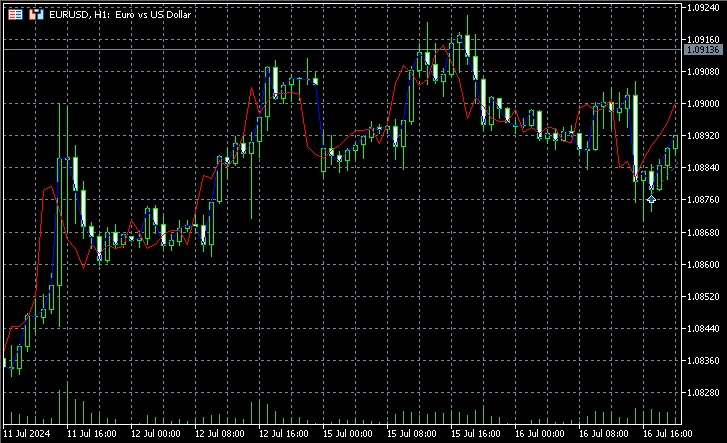
Key aspects of the implementation include the use of a weighted average for prediction, where the weight of each neighbor is inversely proportional to its distance from the current state. This allows us to take into account that closer neighbors are likely to give a more accurate forecast. Judging by the screenshots, the indicator predicts the direction of price movement several bars in advance.

Creating a concept EA

We have reached the most interesting part. Below is the code for fully automated work based on chaos theory:

#property copyright "Copyright 2024, Author"
#property link      "https://www.example.com"
#property version   "1.00"
#property strict

#include <Arrays\ArrayObj.mqh>
#include <Trade\Trade.mqh>
CTrade Trade;
input int    InpEmbeddingDimension = 3;     // Embedding dimension
input int    InpTimeDelay          = 5;     // Time delay
input int    InpNeighbors          = 10;    // Number of neighbors
input int    InpForecastHorizon    = 10;    // Forecast horizon
input int    InpLookback           = 1000;  // Lookback period
input double InpLotSize            = 0.1;   // Lot size

ulong g_ticket = 0;
datetime g_last_bar_time = 0;
double optimalTimeDelay;
double optimalEmbeddingDimension;
int OnInit()
{
   return(INIT_SUCCEEDED);
}

void OnDeinit(const int reason)
{
}

void OnTick()
{  
   OptimizeParameters();
   
   if(g_last_bar_time == iTime(_Symbol, PERIOD_CURRENT, 0)) return;
   g_last_bar_time = iTime(_Symbol, PERIOD_CURRENT, 0);
   
   double prediction = PredictPrice(iClose(_Symbol, PERIOD_CURRENT, 0), 0);
   Comment(prediction);
   
   if(prediction > iClose(_Symbol, PERIOD_CURRENT, 0))
   {
      // Close selling
      for(int i = PositionsTotal() - 1; i >= 0; i--)
      {
         if(PositionGetSymbol(i) == _Symbol && PositionGetInteger(POSITION_TYPE) == POSITION_TYPE_SELL)
         {
            ulong ticket = PositionGetInteger(POSITION_TICKET);
            if(!Trade.PositionClose(ticket))
               Print("Failed to close SELL position: ", GetLastError());
         }
      }
      
      // Open buy
      double ask = SymbolInfoDouble(_Symbol, SYMBOL_ASK);
      ulong ticket = Trade.Buy(InpLotSize, _Symbol, ask, 0, 0, "ChaosBuy");
      if(ticket == 0)
         Print("Failed to open BUY position: ", GetLastError());
   }
   else if(prediction < iClose(_Symbol, PERIOD_CURRENT, 0))
   {
      // Close buying
      for(int i = PositionsTotal() - 1; i >= 0; i--)
      {
         if(PositionGetSymbol(i) == _Symbol && PositionGetInteger(POSITION_TYPE) == POSITION_TYPE_BUY)
         {
            ulong ticket = PositionGetInteger(POSITION_TICKET);
            if(!Trade.PositionClose(ticket))
               Print("Failed to close BUY position: ", GetLastError());
         }
      }
      
      // Open sell
      double bid = SymbolInfoDouble(_Symbol, SYMBOL_BID);
      ulong ticket = Trade.Sell(InpLotSize, _Symbol, bid, 0, 0, "ChaosSell");
      if(ticket == 0)
         Print("Failed to open SELL position: ", GetLastError());
   }
}

double PredictPrice(double price, int index)
{
   int vectorSize = optimalEmbeddingDimension;
   int dataSize = InpLookback;
   
   double currentVector[];
   ArrayResize(currentVector, vectorSize);
   for(int i = 0; i < vectorSize; i++)
   {
      currentVector[i] = iClose(_Symbol, PERIOD_CURRENT, index + i * optimalTimeDelay);
   }
   
   double distances[];
   int indices[];
   ArrayResize(distances, dataSize);
   ArrayResize(indices, dataSize);
   
   for(int i = 0; i < dataSize; i++)
   {
      double dist = 0;
      for(int j = 0; j < vectorSize; j++)
      {
         double diff = currentVector[j] - iClose(_Symbol, PERIOD_CURRENT, index + i + j * optimalTimeDelay);
         dist += diff * diff;
      }
      distances[i] = MathSqrt(dist);
      indices[i] = i;
   }
   
   // Use SortDoubleArray to sort by 'distances' array values
   SortDoubleArray(distances, indices);
   
   double prediction = 0;
   double weightSum = 0;
   
   for(int i = 0; i < InpNeighbors; i++)
   {
      int neighborIndex = index + indices[i];
      double weight = 1.0 / (distances[i] + 0.0001);
      prediction += weight * iClose(_Symbol, PERIOD_CURRENT, neighborIndex + InpForecastHorizon);
      weightSum += weight;
   }
   
   return prediction / weightSum;
}

void SortDoubleArray(double &distances[], int &indices[])
{
    int size = ArraySize(distances);
    for(int i = 0; i < size - 1; i++)
    {
        for(int j = i + 1; j < size; j++)
        {
            if(distances[i] > distances[j])
            {
                // Swap distances
                double tempDist = distances[i];
                distances[i] = distances[j];
                distances[j] = tempDist;
                
                // Swap corresponding indices
                int tempIndex = indices[i];
                indices[i] = indices[j];
                indices[j] = tempIndex;
            }
        }
    }
}

int FindOptimalLagACF(int maxLag, double threshold = 0.1)
{
   int size = InpLookback;
   double series[];
   ArraySetAsSeries(series, true);
   CopyClose(_Symbol, PERIOD_CURRENT, 0, size, series);
   
   double mean = 0;
   for(int i = 0; i < size; i++)
      mean += series[i];
   mean /= size;
   
   double variance = 0;
   for(int i = 0; i < size; i++)
      variance += MathPow(series[i] - mean, 2);
   variance /= size;
   
   for(int lag = 1; lag <= maxLag; lag++)
   {
      double acf = 0;
      for(int i = 0; i < size - lag; i++)
         acf += (series[i] - mean) * (series[i + lag] - mean);
      acf /= (size - lag) * variance;
      
      if(MathAbs(acf) <= threshold)
         return lag;
   }
   
   return maxLag;
}

int FindOptimalEmbeddingDimension(int delay, int maxDim, double threshold = 0.1, double tolerance = 0.01)
{
   int size = InpLookback;
   double series[];
   ArraySetAsSeries(series, true);
   CopyClose(_Symbol, PERIOD_CURRENT, 0, size, series);
   
   for(int dim = 1; dim < maxDim; dim++)
   {
      int falseNeighbors = 0;
      int totalNeighbors = 0;
      
      for(int i = (dim + 1) * delay; i < size; i++)
      {
         int nearestNeighbor = -1;
         double minDist = DBL_MAX;
         
         for(int j = (dim + 1) * delay; j < size; j++)
         {
            if(i == j) continue;
            
            double dist = 0;
            for(int k = 0; k < dim; k++)
            {
               double diff = series[i - k * delay] - series[j - k * delay];
               dist += diff * diff;
            }
            
            if(dist < minDist)
            {
               minDist = dist;
               nearestNeighbor = j;
            }
         }
         
         if(nearestNeighbor != -1)
         {
            totalNeighbors++;
            if(IsFalseNeighbor(series, i, nearestNeighbor, dim, delay, threshold))
               falseNeighbors++;
         }
      }
      
      double fnnRatio = (double)falseNeighbors / totalNeighbors;
      if(fnnRatio < tolerance)
         return dim;
   }
   
   return maxDim;
}

bool IsFalseNeighbor(const double &price[], int index1, int index2, int dim, int delay, double threshold)
{
   double dist1 = 0, dist2 = 0;
   for(int i = 0; i < dim; i++)
   {
      double diff = price[index1 - i * delay] - price[index2 - i * delay];
      dist1 += diff * diff;
   }
   dist1 = MathSqrt(dist1);
   
   double diffNext = price[index1 - dim * delay] - price[index2 - dim * delay];
   dist2 = MathSqrt(dist1 * dist1 + diffNext * diffNext);
   
   return (MathAbs(dist2 - dist1) / dist1 > threshold);
}

void OptimizeParameters()
{
   double optimalTimeDelay = FindOptimalLagACF(50);
   double optimalEmbeddingDimension = FindOptimalEmbeddingDimension(optimalTimeDelay, 10);
   Print("Optimal Time Delay: ", optimalTimeDelay);
   Print("Optimal Embedding Dimension: ", optimalEmbeddingDimension);
}

This code is an EA for MetaTrader 5 that uses chaos theory concepts to forecast prices in financial markets. The EA implements the forecast method based on the nearest neighbor method in the reconstructed phase space.

The EA has the following inputs:

• InpEmbeddingDimension - embedding dimension for phase space reconstruction (default - 3)
• InpTimeDelay - time delay for reconstruction (default - 5)
• InpNeighbors - number of nearest neighbors for forecasting (default - 10)
• InpForecastHorizon - forecast horizon (default - 10)
• InpLookback - lookback period for analysis (default - 1000)
• InpLotSize - lot size for trading (default - 0.1)

The EA works as follows:

1. At each new bar, it optimizes the optimalTimeDelay and optimalEmbeddingDimension parameters using the autocorrelation function (ACF) method and the false nearest neighbors (FNN) algorithm, respectively.
2. It then makes a price prediction based on the current state of the system using the nearest neighbors method.
3. If the price forecast is higher than the current price, the EA closes all open sell positions and opens a new buy position. If the price forecast is lower than the current price, the EA closes all open buy positions and opens a new sell position.

The EA uses the PredictPrice function, which:

• Reconstructs phase space using optimal embedding dimension and time delay.
• Finds the distances between the current state of the system and all states in the lookback period.
• Sorts states by increasing distance.
• Computes a weighted average of future prices for InpNeighbors nearest neighbors, where the weight of each neighbor is inversely proportional to its distance from the current state.
• Returns a weighted average as a price forecast.

The EA also includes the FindOptimalLagACF and FindOptimalEmbeddingDimension functions, which are used to optimize the optimalTimeDelay and optimalEmbeddingDimension parameters, respectively.

Overall, the EA provides an innovative approach to forecasting prices in financial markets using the concepts of chaos theory. It can help traders make more informed decisions and potentially increase investment returns.

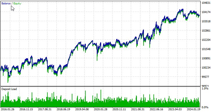
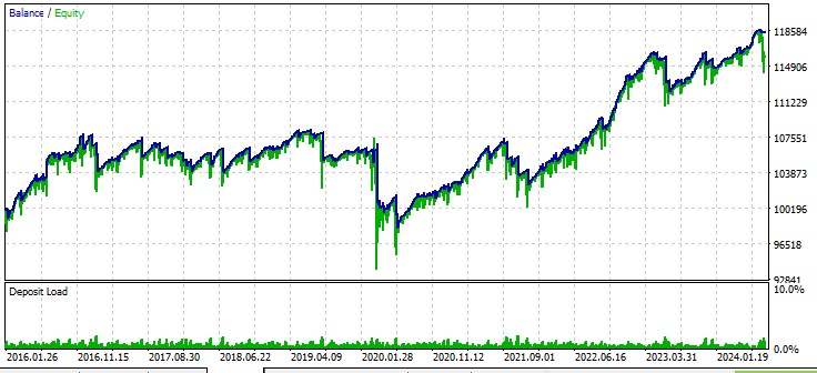
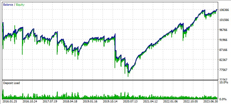
Testing with auto-optimization

Let's consider the work of our EA on several symbols. The first currency pair, EURUSD, period from 01.01.2016:

Second pair, AUD:

Third pair, GBPUSD:

Next steps

Further development of our chaos theory-based EA will require in-depth testing and optimization. Large-scale testing across different timeframes and financial instruments is needed to better understand its efficiency in different market conditions. The use of machine learning methods can help optimize the EA parameters increasing its adaptability to changing market realities.

Particular attention should be paid to improving the risk management system. Implementing dynamic position sizing management, that takes into account current market volatility and chaotic volatility forecasts, may significantly improve the strategy resilience.

Conclusion

In this article, we looked at the application of chaos theory to the analysis and forecasting of financial markets. We studied key concepts such as phase space reconstruction, determining the optimal embedding dimension and time delay, and the nearest neighbor prediction method.

The EA we developed demonstrates the potential of using chaos theory in algorithmic trading. Testing results on various currency pairs show that the strategy is capable of generating profit, although with varying degrees of success on different instruments.

However, it is important to note that applying chaos theory to finance comes with a number of challenges. Financial markets are extremely complex systems influenced by many factors, many of which are difficult or even impossible to take into account in a model. Moreover, the very nature of chaotic systems makes long-term forecasting fundamentally impossible - this is one of the main postulates of serious researchers.

In conclusion, while chaos theory is not the Holy Grail for market forecasting, it does represent a promising direction for further research and development in the fields of financial analysis and algorithmic trading. It is clear that combining chaos theory methods with other approaches, such as machine learning and big data analytics, can open up new possibilities.