
Neural Networks Made Easy (Part 93): Adaptive Forecasting in Frequency and Time Domains (Final Part)

Introduction
In the previous article, we got acquainted with the ATFNet algorithm, which is an ensemble of 2 time series forecasting models. One of them works in the time domain and constructs predictive values of the studied time series based on the analysis of signal amplitudes. The second model works with the frequency characteristics of the analyzed time series and records its global dependencies, their periodicity and spectrum. Adaptive merging of two independent forecasts, according to the author of the method, generates impressive results.
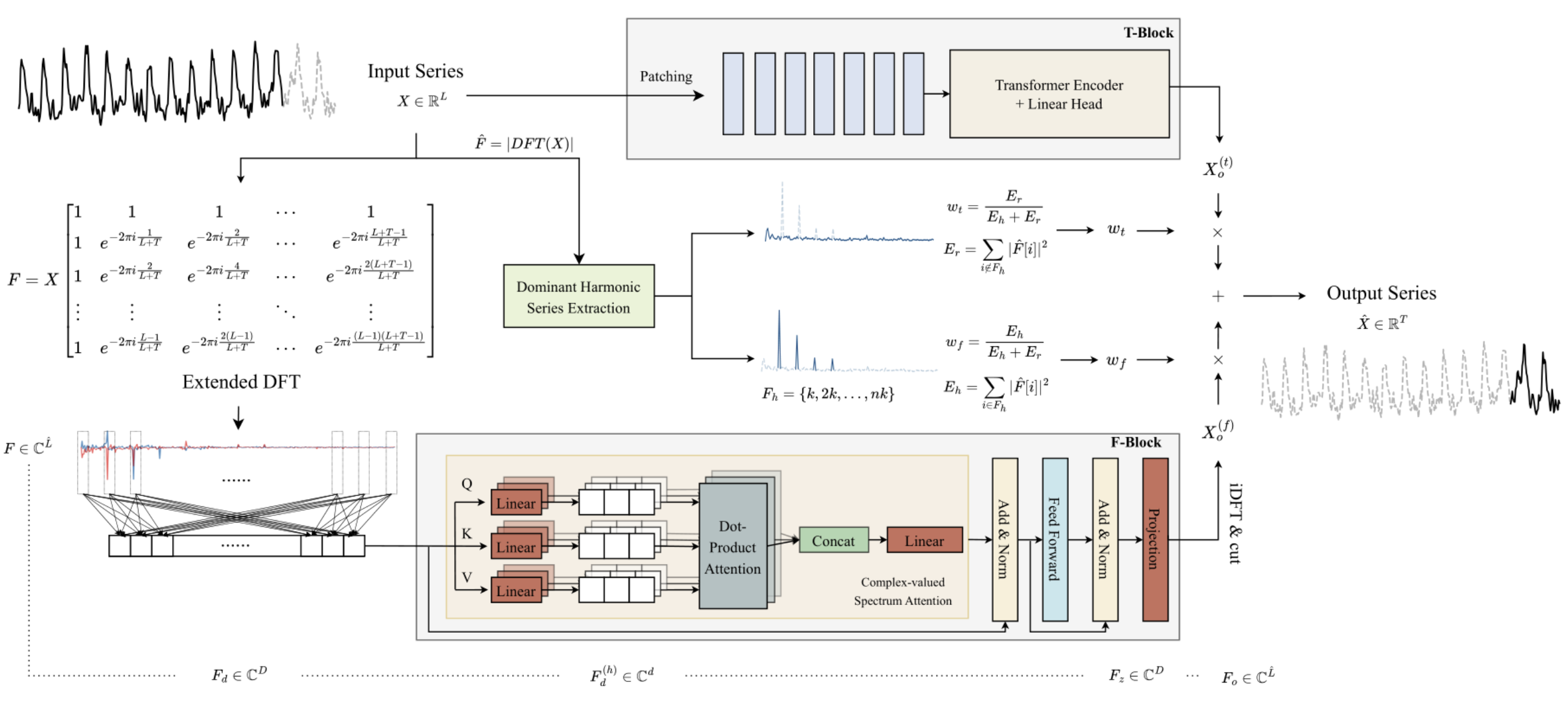
The key feature of the frequency F-Block is a complete construction of the algorithm using the mathematics of complex numbers. To meet this requirement, in the previous article we built the CNeuronComplexMLMHAttention class. It completely repeats the Transformer multilayer Encoder algorithms with elements of multi-headed Self-Attention. The integrated attention class we built is the foundation of the F-Block. In this article, we will continue to implement the approaches proposed by the authors of the ATFNet method.
1. Creating the ATFNet class
After implementing the the foundation of the frequency F-Block, which is the complex attention class CNeuronComplexMLMHAttention, we go up a level and create the CNeuronATFNetOCL class, in which we will implement the entire ATFNet algorithm .
I must admit that the implementation of such a complex algorithm as ATFNet within a single neural layer class may not be the most optimal solution. But the sequential neural network model we built earlier does not provide for the possibility of organizing the work of several different parallel processes, which is exactly our case: we use T-Block and F-Block. The implementation of such functionality will require more global changes. Therefore, I decided to create a solution with minimal costs, i.e. to implement the entire algorithm as one neural layer class. The CNeuronATFNetOCL class structure is shown below.
class CNeuronATFNetOCL  :  public CNeuronBaseOCL
  {
protected:
   uint              iHistory;
   uint              iForecast;
   uint              iVariables;
   uint              iFFT;
   //--- T-Block
   CNeuronBatchNormOCL  cNorm;
   CNeuronTransposeOCL  cTranspose;
   CNeuronPositionEncoder  cPositionEncoder;
   CNeuronPatching      cPatching;
   CLayer               caAttention;
   CLayer               caProjection;
   CNeuronRevINDenormOCL cRevIN;
   //--- F-Block
   CBufferFloat      *cInputs;
   CBufferFloat      cInputFreqRe;
   CBufferFloat      cInputFreqIm;
   CNeuronBaseOCL    cInputFreqComplex;
   CBufferFloat      cMainFreqWeights;
   CNeuronBaseOCL    cNormFreqComplex;
   CBufferFloat      cMeans;
   CBufferFloat      cVariances;
   CNeuronComplexMLMHAttention cFreqAtteention;
   CNeuronBaseOCL    cUnNormFreqComplex;
   CBufferFloat      cOutputFreqRe;
   CBufferFloat      cOutputFreqIm;
   CBufferFloat      cOutputTimeSeriasRe;
   CBufferFloat      cOutputTimeSeriasIm;
   CBufferFloat      cOutputTimeSeriasReGrad;
   CBufferFloat      cReconstructInput;
   CBufferFloat      cForecast;
   CBufferFloat      cReconstructInputGrad;
   CBufferFloat      cForecastGrad;
   CBufferFloat      cZero;
   //---
   virtual bool      FFT(CBufferFloat *inp_re, CBufferFloat *inp_im, CBufferFloat *out_re, CBufferFloat *out_im,
                         bool reverse = false);
   //---
   virtual bool      feedForward(CNeuronBaseOCL *NeuronOCL);
   virtual bool      updateInputWeights(CNeuronBaseOCL *NeuronOCL);
   virtual bool      calcInputGradients(CNeuronBaseOCL *NeuronOCL);
   virtual bool      ComplexNormalize(void);
   virtual bool      ComplexUnNormalize(void);
   virtual bool      ComplexNormalizeGradient(void);
   virtual bool      ComplexUnNormalizeGradient(void);
   virtual bool      MainFreqWeights(void);
   virtual bool      WeightedSum(void);
   virtual bool      WeightedSumGradient(void);
   virtual bool      calcReconstructGradient(void);

public:
                     CNeuronATFNetOCL(void) {};
                    ~CNeuronATFNetOCL(void) {};
   //---
   virtual bool      Init(uint numOutputs, uint myIndex, COpenCLMy *open_cl,
                          uint history, uint forecast, uint variables, uint heads, uint layers, uint &patch[],
                          ENUM_OPTIMIZATION optimization_type, uint batch);
   //---
   virtual int       Type(void)   const   {  return defNeuronATFNetOCL;   }
   //--- methods for working with files
   virtual bool      Save(int const file_handle);
   virtual bool      Load(int const file_handle);
   virtual CLayerDescription* GetLayerInfo(void);
   virtual bool      WeightsUpdate(CNeuronBaseOCL *net, float tau);
   virtual void      SetOpenCL(COpenCLMy *obj);
   virtual CBufferFloat   *getWeights(void);
  };
In the presented CNeuronATFNetOCL class structure, please pay attention to the four internal variables:
- iHistory: the depth of the analyzed history;
- iForecast: planning horizon;
- iVariables: the number of analyzed variables (unitary time series);
- iFFT: the size of the fast Fourier decomposition tensor (DFT).
As we have seen earlier, the DFT algorithm requires the size of the initial data vector to be equal to one of the powers of "2". Therefore, we supplement the initial data tensor with zero values to the required size.
The internal objects of the method are divided into two blocks depending on which block of the ATFNet algorithm they belong to. We will consider their purpose, as well as the functionality of class methods, while implementing the algorithm.
All internal objects are declared statically, and thus we can leave the CNeuronATFNetOCL class constructor and destructor empty.
1.1 Object initialization
Initialization of the internal objects of our new class is performed in the Init method. Here we meet the first consequence of our decision to implement the entire ATFNet algorithm within one class: we need to pass a large number of parameters from the caller.
Actually, within the CNeuronATFNetOCL class, we have to build two parallel multilayer models using attention mechanisms both in the time T-Block and in the frequency F-block. For each of the models, we need to specify the architecture.
To solve this problem, we decided to use "universal" parameters whenever possible, i.e. parameters that can be used equally by both models. Well, we have parameters for describing the input and output tensor: the depth of the analyzed history, the number of unitary time series, and the planning horizon. These parameters are used equally in T-Block and F-Block.
Furthermore, both models are built around the Encoder of the Transformer and exploit the multi-headed Self-Attention architecture with several layers. We decided to use the same number of attention heads and Encoder layers in both blocks.
However, we need to pass additional parameters for the data segmentation layer that is used in T-Block and has no analogue in F-Block. In order not to greatly increase the number of method parameters, I decided to use an array of 3 elements. The first element of this array contains the window size of one segment, and the second element contains the step of this window in the source data buffer. In the last element of the array, we write the size of one patch at the output of the data segmentation layer.
bool CNeuronATFNetOCL::Init(uint numOutputs, uint myIndex, COpenCLMy *open_cl,
                            uint history, uint forecast, uint variables, uint heads, uint layers, uint &patch[],
                            ENUM_OPTIMIZATION optimization_type, uint batch)
  {
   if(!CNeuronBaseOCL::Init(numOutputs, myIndex, open_cl, forecast * variables, optimization_type, batch))
      return false;
In the method body, as usual, we call the parent class initialization method of the same name. Please note that for the parent class method we specify the layer size as the product of the number of analyzed variables (unitary time series) and the planning horizon. In other words, we expect that the output of the CNeuronATFNetOCL layer will be a ready result of the predicted continuation of the analyzed time series.
After successful initialization of the inherited objects, we save key architecture parameters into variables.
   iHistory = MathMax(history, 1);
   iForecast = forecast;
   iVariables = variables;
Then we will calculate the size of the tensor for fast Fourier decomposition. The authors of ATFNet propose an extended Fourier decomposition that determines the frequency characteristics of the full time series given historical and forecast data.
   uint size = iHistory + iForecast;
   int power = int(MathLog(size) / M_LN2);
   if(MathPow(2, power) < size)
      power++;
   iFFT = uint(MathPow(2, power));
The next step is to initialize the internal objects of our class. Let's start with the expected presentation of the initial data. Since our model assumes the analysis of unitary time series in the time and frequency domains, we expect to receive a matrix of unitary time series as the input to our layer. CNeuronATFNetOCL will return a similar map of predicted values at the output.
Another point is data normalization. Both blocks of the model use normalization of the input data. The difference is that T-Block uses normalization in the time domain, and F-block uses in the frequency domain. Therefore, in this implementation, I decided to feed unnormalized data into the layer. Normalization and reverse addition of stochastic characteristics is carried out within individual blocks according to the corresponding dimensions.
For ease of reading and transparency of the code, we will initialize internal objects by blocks of their use and in the order of the constructed algorithm. Let's start with the T-Block.
As mentioned above, unnormalized data is input into the layer. Therefore, we must first convert the obtained data into a comparable form.
//--- T-Block
   if(!cNorm.Init(0, 0, OpenCL, iHistory * iVariables, batch, optimization))
      return false;
The authors of the ATFNetmethod do not use positional data encoding in the frequency domain, but use it when analyzing data in the time domain. Let's add a positional encoding layer.
   if(!cPositionEncoder.Init(0, 1, OpenCL, iVariables, iHistory, optimization, batch))
      return false;
When constructing a data segmentation layer, we built a kind of data transposition into its algorithm. Now we need to prepare the input before feeding it to the CNeuronPatching layer. To perform this operation, we add a data transposition layer.
   if(!cTranspose.Init(0, 2, OpenCL, iHistory, iVariables, optimization, batch))
      return false;
   cTranspose.SetActivationFunction(None);
Next, we need to calculate the number of patches at the output of the segmentation layer based on the window size of one segment and its step, obtained in the method parameters from the external program.
uint count = (iHistory - patch[0] + 2 * patch[1] - 1) / patch[1];
After performing the necessary preparatory work, we initialize the data segmentation layer.
   if(!cPatching.Init(0, 3, OpenCL, patch[0], patch[1], patch[2], count, iVariables, optimization, batch))
      return false;
When constructing the PatchTST method, we used Conformer as an attention block. Here we will use the same solution. In the next step, we create the required number of CNeuronConformer nested layers.
   caAttention.SetOpenCL(OpenCL);
   for(uint l = 0; l < layers; l++)
     {
      CNeuronConformer *temp = new CNeuronConformer();
      if(!temp)
         return false;
      if(!temp.Init(0, 4 + l, OpenCL, patch[2], 32, heads, iVariables, count, optimization, batch))
        {
         delete temp;
         return false;
        }
      if(!caAttention.Add(temp))
        {
         delete temp;
         return false;
        }
     }
The attention block that analyzes the input time series is followed by a block of 3 convolutional layers that will perform forecasting of subsequent data at the entire planning depth in the context of individual unitary time series.
   int total = 3;
   caProjection.SetOpenCL(OpenCL);
   uint window = patch[2] * count;
   for(int l = 0; l < total; l++)
     {
      CNeuronConvOCL *temp = new CNeuronConvOCL();
      if(!temp)
         return false;
      if(!temp.Init(0, 4+layers+l, OpenCL, window, window, (total-l)*iForecast, iVariables, optimization, batch))
        {
         delete temp;
         return false;
        }
      temp.SetActivationFunction(TANH);
      if(!caProjection.Add(temp))
        {
         delete temp;
         return false;
        }
      window = (total - l) * iForecast;
     }
Note that in each layer, we specify the same number of sequence elements, equal to the number of unitary time series in the analyzed time series. In each subsequent layer, the number of filters at the output of the neural layer decreases and becomes equal to the specified prediction depth in the last layer.
At the output of the T-Block, we add to the forecast values statistical parameters of the input time series using the CNeuronRevINDenormOCL layer.
   if(!cRevIN.Init(0, 4 + layers + total, OpenCL, iForecast * iVariables, 1, cNorm.AsObject()))
      return false;
At this point, we have initialized all the internal objects related to the T-Block with the time domain prediction. Now we move on to working with objects of the frequency F-Block.
According to the ATFNet algorithm, input data fed into the F-Block is converted into the frequency domain using fast Fourier decomposition (DFT). As you remember, the implementation of the DFT algorithm we built earlier writes the frequency spectrum into two data buffers. One for the real part of the spectrum, the second for the imaginary part.
//--- F-Block
   if(!cInputFreqRe.BufferInit(iFFT * iVariables, 0) || !cInputFreqRe.BufferCreate(OpenCL))
      return false;
   if(!cInputFreqIm.BufferInit(iFFT * iVariables, 0) || !cInputFreqIm.BufferCreate(OpenCL))
      return false;
For ease of subsequent processing, we will combine the spectrum information into one buffer.
   if(!cInputFreqComplex.Init(0, 0, OpenCL, iFFT * iVariables * 2, optimization, batch))
      return false;
We also need to prepare a buffer for writing the share of the dominant frequency. It should be noted here that we determine the dominant frequency separately for each unitary time series.
   if(!cMainFreqWeights.BufferInit(iVariables, 0) || !cMainFreqWeights.BufferCreate(OpenCL))
      return false;
The input to our layer is raw data, which generates quite different spectra of unitary time series. To convert the spectra into a comparable form before subsequent processing, the authors of the method recommend normalizing the frequency characteristics. We will save normalized data in cNormFreqComplex layer buffers.
   if(!cNormFreqComplex.Init(0, 1, OpenCL, iFFT * iVariables * 2, optimization, batch))
      return false;
In this case, we will save the statistical characteristics of the original spectrum in the corresponding data buffers.
   if(!cMeans.BufferInit(iVariables, 0) || !cMeans.BufferCreate(OpenCL))
      return false;
   if(!cVariances.BufferInit(iVariables, 0) || !cVariances.BufferCreate(OpenCL))
      return false;
We will process the frequency characteristics of the prepared input data using the complex attention block. In the previous article, we performed a big implementation of the CNeuronComplexMLMHAttention class. Now we just need to initialize the internal object of the specified class.
   if(!cFreqAtteention.Init(0, 2, OpenCL, iFFT, 32, heads, iVariables, layers, optimization, batch))
      return false;
According to the algorithm, after processing the input spectrum in the complex attention block, we need to execute inverse procedures. First, we add statistical indicators of the input frequency characteristics to the processed spectrum.
   if(!cUnNormFreqComplex.Init(0, 1, OpenCL, iFFT * iVariables * 2, optimization, batch))
      return false;
Let's separate the real and imaginary parts of the spectrum.
   if(!cOutputFreqRe.BufferInit(iFFT*iVariables, 0) || !cOutputFreqRe.BufferCreate(OpenCL))
      return false;
   if(!cOutputFreqIm.BufferInit(iFFT*iVariables, 0) || !cOutputFreqIm.BufferCreate(OpenCL))
      return false;
Then we return the data to the temporary area.
   if(!cOutputTimeSeriasRe.BufferInit(iFFT*iVariables, 0) || !cOutputTimeSeriasRe.BufferCreate(OpenCL))
      return false;
   if(!cOutputTimeSeriasIm.BufferInit(iFFT*iVariables, 0) || !cOutputTimeSeriasIm.BufferCreate(OpenCL))
      return false;
For the purposes of the backpropagation pass, we create a gradient buffer for the real part of the time series.
   if(!cOutputTimeSeriasReGrad.BufferInit(iFFT*iVariables, 0) || !cOutputTimeSeriasReGrad.BufferCreate(OpenCL))
      return false;
Please note that we do not create a gradient buffer for the imaginary part of the time series. The point is that for a time series, the target values of the imaginary part are "0". Therefore, the error gradient of the imaginary part is equal to the values of the imaginary part with the opposite sign. In the backpropagation pass, we can use the feed-forward pass results buffer for the imaginary part of the processed time series.
Please note that after the inverse DFT (iDFT), we plan to receive a processed full time series consisting of a reconstruction of the input data and forecast values for a given planning horizon. To extract the required portion of the forecast values, we divide the full time series into two buffers: reconstructed data and forecast values.
   if(!cReconstructInput.BufferInit(iHistory*iVariables, 0) || !cReconstructInput.BufferCreate(OpenCL))
      return false;
   if(!cForecast.BufferInit(iForecast*iVariables, 0) || !cForecast.BufferCreate(OpenCL))
      return false;
Add buffers for the corresponding error gradients.
   if(!cReconstructInputGrad.BufferInit(iHistory*iVariables, 0) || !cReconstructInputGrad.BufferCreate(OpenCL))
      return false;
   if(!cForecastGrad.BufferInit(iForecast*iVariables, 0) || !cForecastGrad.BufferCreate(OpenCL))
      return false;
Please note that the method proposed by the ATFNet authors provides no analysis of deviations of the reconstructed data from the input values of the analyzed time series. We add this functionality in an attempt to implement a more fine-tuned adjustment of the complex attention block. Potentially, a better understanding of the data being analyzed will improve the model's prediction quality.
Additionally, we create a buffer of zero values that will be used to fill in missing values in the input data and error gradients.
   if(!cZero.BufferInit(iFFT*iVariables, 0) || !cZero.BufferCreate(OpenCL))
      return false;
//---
   return true;
  }
Do not forget to monitor the operations processes at every stage. After the initialization of all declared objects is complete, we return the logical value of the execution of the method operations to the caller.
1.2 Feed-forward pass
After completing the initialization of class objects, we move on to constructing the feed-forward algorithm. Let's start with building additional kernels in the OpenCL program.
First, think about the normalization of frequency response spectra of unitary time series. If we use previously implemented real data normalization algorithms, this can greatly distort the data. Therefore, we need to implement data normalization in a complex domain. We implement this functionality in the ComplexNormalize kernel. In the kernel parameters, we will pass pointers to 4 data buffers and the size of the unitary sequence. We will use this kernel in a one-dimensional problem space in the context of unitary time series spectra.
__kernel void ComplexNormalize(__global float2 *inputs,
                               __global float2 *outputs,
                               __global float2 *means,
                               __global float *vars,
                               int dimension)
  {
   if(dimension <= 0)
      return;
Note the declaration of data buffers. The input, output and mean data buffers are of vector type float2. We decided to use this type of data on the OpenCL side for working with complex quantities. However, there is also a dispersions buffer that is declared with a real type float. Dispersions show the standard deviation of a value from the mean. The distance between two points is a real quantity.
In the body of the method, we check the obtained dimension of the normalized vector. Obviously, it must be greater than "0". We then identify the current thread in the task space, determine the offset in the data buffers, and create a complex representation of the dimensionality of the sequence being analyzed.
   size_t n = get_global_id(0);
   const int shift = n * dimension;
   const float2 dim = (float2)(dimension, 0);
Next, we organize a loop in which we determine the average value of the analyzed spectrum.
   float2 mean = 0;
   for(int i = 0; i < dimension; i++)
     {
      float2 val = inputs[shift + i];
      if(isnan(val.x) || isinf(val.x) ||
         isnan(val.y) || isinf(val.y))
         inputs[shift + i] = (float2)0;
      else
         mean += val;
     }
   means[n] = mean = ComplexDiv(mean, dim);
We immediately save the obtained result in the corresponding element of the average value buffer.
At the next stage, we organize a loop for determining the dispersion of the analyzed sequence.
   float variance = 0;
   for(int i = 0; i < dimension; i++)
      variance += pow(ComplexAbs(inputs[shift + i] - mean), 2);
   vars[n] = variance = sqrt((isnan(variance) || isinf(variance) ? 1.0f : variance / dimension));
There are two points to note here. First, despite saving the average value in the external data buffer, we use the value of the local variable when performing operations, since accessing a buffer element located in the global memory of the context is much slower than accessing a local kernel variable.
The second point is methodical: when calculating the variance of a sequence of complex numbers, unlike real numbers, we square the absolute value of the deviation of an element of the complex sequence from the mean value. It is the absolute value of a complex quantity that will show the distance between points in the 2-dimensional space of the real and imaginary parts. While a simple difference of complex quantities will only show us a shift in coordinates.
At the last stage of the kernel operation, we organize the last loop, in which we normalize the data of the input spectrum. We write the obtained values into the corresponding elements of the result buffer.
   float2 v=(float2)(variance, 0);
   for(int i = 0; i < dimension; i++)
     {
      float2 val = ComplexDiv((inputs[shift + i] - mean), v);
      if(isnan(val.x) || isinf(val.x) || isnan(val.y) || isinf(val.y))
         val = (float2)0;
      outputs[shift + i] = val;
     }
  }
Here we also work with local variables of mean and standard deviation.
And we will immediately create a reverse normalization kernel ComplexUnNormalize, in which we return the extracted statistical indicators of the input spectrum.
__kernel void ComplexUnNormalize(__global float2 *inputs,
                                 __global float2 *outputs,
                                 __global float2 *means,
                                 __global float *vars,
                                 int dimension)
  {
   if(dimension <= 0)
      return;
This kernel receives the same set of parameters of 4 pointers to data buffers and one variable. We also plan to run the kernel in a 1-dimensional task space for the number of unitary time series.
In the kernel body, we identify the thread in the task space and define offsets in the data buffers.
   size_t n = get_global_id(0);
   const int shift = n * dimension;
Load statistical variables from the buffers and immediately convert the standard deviation into a complex value.
   float v= vars[n];
   float2 variance=(float2)((v > 0 ? v : 1.0f), 0)
   float2 mean = means[n];
Then organize the only data conversion loop in this kernel.
   for(int i = 0; i < dimension; i++)
     {
      float2 val = ComplexMul(inputs[shift + i], variance) + mean;
      if(isnan(val.x) || isinf(val.x) || isnan(val.y) || isinf(val.y))
         val = (float2)0;
      outputs[shift + i] = val;
     }
  }
The obtained values are written to the corresponding elements of the result buffer.
To call the above-created kernels on the main program side, we use ComplexNormalize and ComplexUnNormalize methods. The algorithm for their construction does not differ from the previously considered methods for enqueuing the kernels of the OpenCL program. Therefore, we will not dwell on these methods. Anyway, they are provided in the attachment.
In addition, to adaptively combine the results of time and frequency forecasting, we need influence coefficients. The authors of the ATFNet method propose to determine them by the share of the dominant frequency in the overall spectrum. Accordingly, on the OpenCL side we will create two kernels for the program:
- MainFreqWeight — determine the share of the dominant frequency;
- WeightedSum — compute the weighted sum of forecasts in the frequency and time domains.
We plan both kernels in a 1-dimensional task space according to the number of analyzed unitary time series.
In the MainFreqWeight kernel parameters, we pass pointers to two data buffers (frequency characteristics and results) and the dimension of the analyzed series.
__kernel void MainFreqWeight(__global float2 *freq,
                             __global float *weight,
                             int dimension
                            )
  {
   if(dimension <= 0)
      return;
//---
   size_t n = get_global_id(0);
   const int shift = n * dimension;
In the kernel body, we identify the current thread in the task space and determine the offsets in the data buffers. After that we prepare local variables.
   float max_f = 0;
   float total = 0;
   float energy;
Next we run a loop to determine the energy of the dominant frequency and the entire spectrum.
   for(int i = 0; i < dimension; i++)
     {
      energy = ComplexAbs(freq[shift + i]);
      total += energy;
      max_f = fmax(max_f, energy);
     }
To complete the kernel operations, we divide the dominant frequency energy by the total spectrum energy. The resulting value is saved in the corresponding element of the output buffer.
   weight[n] = max_f / (total > 0 ? total : 1);
  }
The algorithm of the WeightedSum kernel for determining the weighted sum of time and frequency domain predictions is quite simple. In the parameters, the kernel receives 4 pointers to data buffers and the dimension of the vector of one sequence (in our case, the prediction depth).
__kernel void WeightedSum(__global float *inputs1,
                          __global float *inputs2,
                          __global float *outputs,
                          __global float *weight,
                          int dimension
                         )
  {
   if(dimension <= 0)
      return;
//---
   size_t n = get_global_id(0);
   const int shift = n * dimension;
In the kernel body, we identify the current thread in the one-dimensional task space and determine the offsets in the data buffers: Then we create a loop of weighted summation of elements. The results of the operations are written to the corresponding element of the result buffer.
   float w = weight[n];
   for(int i = 0; i < dimension; i++)
      outputs[shift + i] = inputs1[shift + i] * w + inputs2[shift + i] * (1 - w);
  }
To place kernels in the execution queue on the main program side, we create methods of the same name. You will find these codes in the attachment.
After completing the preparatory work, we move on to constructing the feed-forward pass method feedForward of our CNeuronATFNetOCL class. In the parameters of this method, as well as the similar method of the parent class, we receive a pointer to the object of the previous neural layer, which in this case acts as the initial data for subsequent operations.
bool CNeuronATFNetOCL::feedForward(CNeuronBaseOCL *NeuronOCL)
  {
   if(!NeuronOCL || !NeuronOCL.getOutput())
      return false;
In the method body, we first check the relevance of the received pointer. Here we also save a pointer to the result buffer of the obtained neural layer in the internal variable of the current object.
   if(cInputs != NeuronOCL.getOutput())
      cInputs = NeuronOCL.getOutput();
Next, we first perform forecasting operations on subsequent data of the analyzed time series in the time domain. Normalize the obtained data.
//--- T-Block
   if(!cNorm.FeedForward(NeuronOCL))
      return false;;
Then add positional encoding.
   if(!cPositionEncoder.FeedForward(cNorm.AsObject()))
      return false;
Transpose the resulting tensor and split the data into patches.
   if(!cTranspose.FeedForward(cPositionEncoder.AsObject()))
      return false;
   if(!cPatching.FeedForward(cTranspose.AsObject()))
      return false;
The prepared data passes through the attention block.
   int total = caAttention.Total();
   CNeuronBaseOCL *prev = cPatching.AsObject();
   for(int i = 0; i < total; i++)
     {
      CNeuronBaseOCL *att = caAttention.At(i);
      if(!att.FeedForward(prev))
         return false;
      prev = att;
     }
Subsequent values are predicted.
   total = caProjection.Total();
   for(int i = 0; i < total; i++)
     {
      CNeuronBaseOCL *proj = caProjection.At(i);
      if(!proj.FeedForward(prev))
         return false;
      prev = proj;
     }
At the output of the T-block, we add statistical values of the input time series to the forecast values.
   if(!cRevIN.FeedForward(prev))
      return false;
After obtaining the predicted values in the time domain, we move on to working with the frequency domain. First, we transform the obtained time series into a spectrum of frequency characteristics. For this we use the FFT algorithm.
//--- F-Block
   if(!FFT(cInputs, cInputs, GetPointer(cInputFreqRe), GetPointer(cInputFreqIm), false))
      return false;
After obtaining two buffers of the real and imaginary parts of the frequency spectrum, we combine them into a single tensor.
   if(!Concat(GetPointer(cInputFreqRe), GetPointer(cInputFreqIm), cInputFreqComplex.getOutput(), 1, 1,
                                                                                     iFFT * iVariables))
      return false;
Note that when concatenating for both data buffers we use a window size of 1 element. Thus, we obtain a tensor in which the real and imaginary parts of the corresponding frequency characteristic are close together.
We normalize the resulting tensor of input frequency.
   if(!ComplexNormalize())
      return false;
Determine the share of the dominant frequency.
   if(!MainFreqWeights())
      return false;
We pass the prepared frequency data through the attention block. Here we only need to call the feed-forward pass method of the multilayer complex attention class created in the previous article.
   if(!cFreqAtteention.FeedForward(cNormFreqComplex.AsObject()))
      return false;
After successful execution of the attention block operations, we return the statistical parameters the input series frequency to the processed data.
   if(!ComplexUnNormalize())
      return false;
Divide the frequency spectrum tensor into its constituent real and imaginary parts.
   if(!DeConcat(GetPointer(cOutputFreqRe), GetPointer(cOutputFreqIm), cUnNormFreqComplex.getOutput(), 1, 1,
                                                                                          iFFT * iVariables))
      return false;
Transform the frequency spectrum back into a time series.
   if(!FFT(GetPointer(cOutputFreqRe), GetPointer(cOutputFreqIm),

           GetPointer(cOutputTimeSeriasRe), GetPointer(cOutputTimeSeriasIm), true))
      return false;
I think we should explain the above operations of the F-Block. At first glance, it may seem strange to perform a large number of transformations of a time series into frequency responses, normalize them, and then perform inverse operations returning the data to the same time series, just to perform attention operations. Moreover, all these operations, except for attention, do not have trainable parameters and should theoretically return the original time series. But it's all about the attention block.
Let me remind you that the authors of the method proposed using the extended discrete Fourier transform. In practice, we simply use a complex exponential basis for a DFT of a complete time series. But when transforming the original time series into its frequency feature, we do not have predicted values and simply replace them with zero values. Therefore, the execution of an inverse DFT quite expectedly will return predicted values close to "0", which is not adequate. Therefore, we bring the spectra of unitary time series into a comparable form by normalizing them. By comparing them with each other in the attention block, we try to teach the model to restore the missing data of the analyzed frequency characteristics.
Thus, at the output of the complex attention block, we expect to receive modified and mutually consistent spectra of frequency characteristics of unitary complete time series with restored missing data. By restoring the time series from the modified spectra, we can obtain forecast values of the analyzed time series that differ from zero.
To complete the feed-forward pass operations, we just need to extract the predicted values from the full time series.
   if(!DeConcat(GetPointer(cReconstructInput), GetPointer(cForecast), GetPointer(cOutputTimeSeriasReGrad),

                GetPointer(cOutputTimeSeriasRe), iHistory, iForecast, iFFT - iHistory - iForecast, iVariables))
      return false;
And add up the predictions made in the time and frequency domains, taking into account the significance coefficient.
//--- Output
   if(!WeightedSum())
      return false;
//---
   return true;
  }
Don't forget to monitor the results of the operations at every stage. After the method operations are completed, we return the logical result of all operations to the caller.
1.3 Error gradient distribution
After performing the feed-forward pass, we need to distribute the error gradient to all training parameters of the model. In our new class, they are both in T-Block and in the F-Block. Therefore, we need to implement a mechanism for propagating the error gradient through T and F blocks. Then we need to combine the error gradient from the two streams and pass the resulting gradient to the previous layer.
As with the feed-forward pass, before constructing the calcInputGradients method, we need to do some preparatory work. During the feed-forward pass, on the OpenCL side, we created kernels for normalization and reverse return of statistical distribution values: ComplexNormalize and ComplexUnNormalize. In the backpropagation pass, we need to create error gradient distribution kernels through the specified operations ComplexNormalizeGradient and ComplexUnNormalizeGradient, respectively.
In the error gradient distribution kernel, through the frequency normalization block, we only divide the obtained error gradient by the standard deviation of the corresponding spectrum.
__kernel void ComplexNormalizeGradient(__global float2 *inputs_gr,
                                       __global float2 *outputs_gr,
                                       __global float *vars,
                                       int dimension)
  {
   if(dimension <= 0)
      return;
//---
   size_t n = get_global_id(0);
   const int shift = n * dimension;
//---
   float v = vars[n];
   float2 variance = (float2)((v > 0 ? v : 1.0f), 0);
   for(int i = 0; i < dimension; i++)
     {
      float2 val = ComplexDiv(outputs_gr[shift + i], variance);
      if(isnan(val.x) || isinf(val.x) || isnan(val.y) || isinf(val.y))
         val = (float2)0;
      inputs_gr[shift + i] = val;
     }
  }
I must say that this is a rather simplified approach to solving this problem. Here we take the mean value and standard deviation as constants. In fact they are functions, and according to the rules of gradient descent we also need to adjust for their influence and propagate the error gradient to the influencing elements of the model. But as practice shows, the influence of these elements on the initial data is quite small. So, to reduce the model training cost, we will omit these operations.
The kernel for the gradient distribution through data denormalization operations is similar, with the only difference that here we multiply the resulting error gradient by the standard deviation.
__kernel void ComplexUnNormalizeGradient(__global float2 *inputs_gr,
      __global float2 *outputs_gr,
      __global float *vars,
      int dimension)
  {
   if(dimension <= 0)
      return;
//---
   size_t n = get_global_id(0);
   const int shift = n * dimension;
//---
   float v = vars[n];
   float2 variance = (float2)((v > 0 ? v : 1.0f), 0);
   for(int i = 0; i < dimension; i++)
     {
      float2 val = ComplexMul(outputs_gr[shift + i], variance);
      if(isnan(val.x) || isinf(val.x) || isnan(val.y) || isinf(val.y))
         val = (float2)0;
      inputs_gr[shift + i] = val;
     }
  }
Next, we need to implement a kernel to distribute the total error gradient between prediction blocks in the time and frequency domains. We implement this functionality in the WeightedSumGradient kernel. In the parameters, this kernel receives pointers to 4 data buffers and 1 parameter, similar to the corresponding feed-forward kernel.
__kernel void WeightedSumGradient(__global float *inputs_gr1,
                                  __global float *inputs_gr2,
                                  __global float *outputs_gr,
                                  __global float *weight,
                                  int dimension
                                 )
  {
   if(dimension <= 0)
      return;
//---
   size_t n = get_global_id(0);
   const int shift = n * dimension;
In the kernel body, we, as usual, identify the current thread in the one-dimensional task space and determine the offset in data buffers. After that, we will prepare local weight variables for the frequency and time series forecasts.
   float w = weight[n];
   float w1 = 1 - weight[n];
Then we create a loop to propagate the error gradient across the corresponding data buffers.
   for(int i = 0; i < dimension; i++)
     {
      float grad = outputs_gr[shift + i];
      inputs_gr1[shift + i] = grad * w;
      inputs_gr2[shift + i] = grad * w1;
     }
  }
The above error gradient propagation kernels are placed in the execution queue within the relevant methods on the main program side. You can familiarize yourself with the code of these methods in the attachment.
Another point we should pay attention to is the calculation of the error gradient of the reconstructed time series of historical values. We will implement this functionality in the calcReconstructGradient method.
Although the operations are performed on the OpenCL context side, to perform the specified operations we do not create a new kernel. Instead, we will use a ready-made kernel determining the error gradient based on target values. We just need to create a method to put the kernel into the execution queue using the data buffers of our F-Block.
The kernel we use runs in a one-dimensional task space according to the number of elements in the tensor. In our case, the size of the analyzed vector is equal to the product of the depth of the analyzed history and the number of unitary time series.
bool CNeuronATFNetOCL::calcReconstructGradient(void)
  {
   uint global_work_offset[1] = {0};
   uint global_work_size[1];
   global_work_size[0] = iHistory * iVariables;
Our target data includes the values of the original data that we obtained during the feed-forward pass from the previous neural layer. During the feed-forward pass, we saved a pointer to the data buffer we needed.
   if(!OpenCL.SetArgumentBuffer(def_k_CalcOutputGradient, def_k_cog_matrix_t, cInputs.GetIndex()))
     {
      printf("Error of set parameter kernel %s: %d; line %d", __FUNCTION__, GetLastError(), __LINE__);
      return false;
     }
We determine the error gradient for the reconstructed data from the processed spectrum.
   if(!OpenCL.SetArgumentBuffer(def_k_CalcOutputGradient, def_k_cog_matrix_o, cReconstructInput.GetIndex()))
     {
      printf("Error of set parameter kernel %s: %d; line %d", __FUNCTION__, GetLastError(), __LINE__);
      return false;
     }
We will write the results of the operations into the gradient buffer of the recovered data.
   if(!OpenCL.SetArgumentBuffer(def_k_CalcOutputGradient, def_k_cog_matrix_ig, cReconstructInputGrad.GetIndex()))
     {
      printf("Error of set parameter kernel %s: %d; line %d", __FUNCTION__, GetLastError(), __LINE__);
      return false;
     }
We did not use activation functions in the forward pass.
   if(!OpenCL.SetArgument(def_k_CalcOutputGradient, def_k_cog_activation, (int)None))
     {
      printf("Error of set parameter kernel %s: %d; line %d", __FUNCTION__, GetLastError(), __LINE__);
      return false;
     }
We put the kernel in the execution queue, check the result of the operations and complete the method, returning the logical result of the operations performed to the caller.
   if(!OpenCL.SetArgument(def_k_CalcOutputGradient, def_k_cog_error, 1))
     {
      printf("Error of set parameter kernel %s: %d; line %d", __FUNCTION__, GetLastError(), __LINE__);
      return false;
     }
   ResetLastError();
   if(!OpenCL.Execute(def_k_CalcOutputGradient, 1, global_work_offset, global_work_size))
     {
      printf("Error of execution kernel CalcOutputGradient: %d", GetLastError());
      return false;
     }
//---
   return true;
  }
After completing the preparatory work, we proceed directly to the construction of the error gradient propagation method calcInputGradients.
In the parameters of this method, similar to the same method of the parent class, we receive a pointer to the object of the previous neural layer, to which we must propagate the error gradient.
bool CNeuronATFNetOCL::calcInputGradients(CNeuronBaseOCL *NeuronOCL)
  {
   if(!NeuronOCL || !NeuronOCL.getGradient() || !cInputs)
      return false;
In the body of the method, we immediately check the relevance of the received pointer. After that, we distribute the error gradient obtained from the subsequent layer into 2 streams between the prediction blocks in the time and frequency domains.
//--- Output
   if(!WeightedSumGradient())
      return false;
First, we propagate the error gradient through the time domain prediction T-Block. Here, in the order reverse to the feed-forward pass, we call the relevant methods of the nested objects.
//--- T-Block
   if(cRevIN.Activation() != None &&
     !DeActivation(cRevIN.getOutput(), cRevIN.getGradient(), cRevIN.getGradient(), cRevIN.Activation()))
      return false;
   CNeuronBaseOCL *next = cRevIN.AsObject();
   for(int i = caProjection.Total() - 1; i >= 0; i--)
     {
      CNeuronBaseOCL *proj = caProjection.At(i);
      if(!proj || !proj.calcHiddenGradients((CObject *)next))
         return false;
      next = proj;
     }
   for(int i = caAttention.Total() - 1; i >= 0; i--)
     {
      CNeuronBaseOCL *att = caAttention.At(i);
      if(!att || !att.calcHiddenGradients((CObject *)next))
         return false;
      next = att;
     }
   if(!cPatching.calcHiddenGradients((CObject*)next))
      return false;
   if(!cTranspose.calcHiddenGradients(cPatching.AsObject()))
      return false;
   if(!cPositionEncoder.calcHiddenGradients(cTranspose.AsObject()))
      return false;
   if(!cNorm.calcHiddenGradients(cPositionEncoder.AsObject()))
      return false;
   if(!NeuronOCL.calcHiddenGradients(cNorm.AsObject()))
      return false;
The gradient propagation algorithm in the frequency prediction block is a bit more complicated. Here we first define the error gradient for the imaginary part of the reconstructed time series. As mentioned earlier, the target value for the imaginary part of the time series is 0. Therefore, to determine the error gradient, we simply change the sign of the feed-forward pass results.
//--- F-Block
   if(!CNeuronBaseOCL::SumAndNormilize(GetPointer(cOutputTimeSeriasIm), GetPointer(cOutputTimeSeriasIm),
                                       GetPointer(cOutputTimeSeriasIm), iFFT*iVariables, false, 0, 0, 0, -0.5))
      return false;
Next, we define the gradient of the historical data recovery error.
   if(!calcReconstructGradient())
      return false;
After that we combine the gradient tensors of the historical data recovery error (defined in the calcReconstructGradient method), the time series forecast error gradient (obtained by dividing the gradient of the error of the subsequent layer into two streams) and supplement it with zero values up to the size of the spectrum of the full series.
   if(!Concat(GetPointer(cReconstructInputGrad), GetPointer(cForecastGrad), GetPointer(cZero),
              GetPointer(cOutputTimeSeriasReGrad), iHistory, iForecast, iFFT - iHistory - iForecast, iVariables))
      return false;
We append zero values to the end of the error gradient tensor of the full time series, since we have no data on target values beyond the planning horizon. This means that we simply don't correct them.
The resulting error gradient for the full time series constructed using the frequency prediction block data is translated into the frequency domain by applying FFT.
   if(!FFT(GetPointer(cOutputTimeSeriasReGrad), GetPointer(cOutputTimeSeriasIm),


           GetPointer(cOutputFreqRe), GetPointer(cOutputFreqIm), false))
      return false;
We combine the obtained data of the real and imaginary parts of the frequency spectrum of the error gradient into a single tensor.
   if(!Concat(GetPointer(cOutputFreqRe), GetPointer(cOutputFreqIm), cUnNormFreqComplex.getGradient(),
                                                                              1, 1, iFFT * iVariables))
      return false;
Correct the error gradient for the derivative of the data denormalization operations.
   if(!ComplexUnNormalizeGradient())
      return false;
Propagate the error gradient through the complex attention block.
   if(!cNormFreqComplex.calcHiddenGradients(cFreqAtteention.AsObject()))
      return false;
Then correct the error gradient by the derivative of the data normalization function.
   if(!ComplexNormalizeGradient())
      return false;
Separate the real and imaginary parts of the spectrum.
   if(!DeConcat(GetPointer(cInputFreqRe), GetPointer(cInputFreqIm), cInputFreqComplex.getGradient(),
                                                                             1, 1, iFFT * iVariables))
      return false;
Return the error gradient to the time domain using IFFT.
   if(!FFT(GetPointer(cInputFreqRe), GetPointer(cInputFreqIm),


           GetPointer(cOutputTimeSeriasRe), GetPointer(cOutputTimeSeriasIm), false))
      return false;
Note that we obtained the error gradient for the full time series. But we only need to propagate the gradient of the error of the historical data to the previous layer. Therefore, we first select the data for the historical horizon under analysis.
   if(!DeConcat(GetPointer(cInputFreqRe), GetPointer(cOutputTimeSeriasIm), GetPointer(cOutputTimeSeriasRe),
                                                                        iHistory, iFFT-iHistory, iVariables))
      return false;
Then we add the obtained values to the results of the error gradient distribution of the T-Block.
   if(!CNeuronBaseOCL::SumAndNormilize(NeuronOCL.getGradient(), GetPointer(cInputFreqRe),
                                       NeuronOCL.getGradient(), iHistory*iVariables, false, 0, 0, 0, 0.5))
      return false;
//---
   return true;
  }
As always, at each iteration we control the process of performing operations. After successful completion of all operations, we return the logical result of the method to the caller.
1.4 Updating model parameters
The error gradient of each trained parameter of the model determines its influence on the overall result. In the next step, we adjust the model parameters to minimize the error. This functionality is performed in the updateInputWeights method. Within the implementation of our class, updating parameters indicates calling the same-name methods of nested objects containing the parameters being trained. In F-Block, it is only a complex attention class.
bool CNeuronATFNetOCL::updateInputWeights(CNeuronBaseOCL *NeuronOCL)
  {
//--- F-Block
   if(!cFreqAtteention.UpdateInputWeights(cNormFreqComplex.AsObject()))
      return false;
The T-Block has more such objects.
//--- T-Block
   if(!cPatching.UpdateInputWeights(cPositionEncoder.AsObject()))
      return false;
   int total = caAttention.Total();
   CNeuronBaseOCL *prev = cPatching.AsObject();
   for(int i = 0; i < total; i++)
     {
      CNeuronBaseOCL *att = caAttention.At(i);
      if(!att.UpdateInputWeights(prev))
         return false;
      prev = att;
     }
   total = caProjection.Total();
   for(int i = 0; i < total; i++)
     {
      CNeuronBaseOCL *proj = caProjection.At(i);
      if(!proj.UpdateInputWeights(prev))
         return false;
      prev = proj;
     }
//---
   return true;
  }
This concludes our consideration of the algorithms for implementing the approaches proposed by the authors of the ATFNet method. You can find the complete code of the CNeuronATFNetOCL class in the attachment.
2. Model architecture
We have completed our class that implements the approaches of the ATFNet method. Let's move on to building the architecture of our models. As you may have already guessed, we will be implementing a new neural layer in the Environment State Encoder. Of course, it's difficult to refer to the CNeuronATFNetOCL class as a neural layer. It implements a rather complex architecture for constructing a comprehensive model.
We will feed our encoder with a set of raw inputs, as we did with the previously constructed models.
bool CreateEncoderDescriptions(CArrayObj *encoder)
  {
//---
   CLayerDescription *descr;
//---
   if(!encoder)
     {
      encoder = new CArrayObj();
      if(!encoder)
         return false;
     }
//--- Encoder
   encoder.Clear();
//--- Input layer
   if(!(descr = new CLayerDescription()))
      return false;
   descr.type = defNeuronBaseOCL;
   int prev_count = descr.count = (HistoryBars * BarDescr);
   descr.activation = None;
   descr.optimization = ADAM;
   if(!encoder.Add(descr))
     {
      delete descr;
      return false;
     }
However, in this case we do not normalize the obtained data. Both the T-Block and the F-Block have data normalization in their architectures. So we skip this step. However, our inputs are formed according to vectors describing individual states of the environment. Before further processing, we transpose the inputs to enable analysis in terms of unitary time series.
//--- layer 1
   if(!(descr = new CLayerDescription()))
      return false;
   descr.type = defNeuronTransposeOCL;
   descr.count = HistoryBars;
   descr.window = BarDescr;
   if(!encoder.Add(descr))
     {
      delete descr;
      return false;
     }
Next, we use our new class to forecast subsequent data in the analyzed time series.
//--- layer 2
   if(!(descr = new CLayerDescription()))
      return false;
   descr.type = defNeuronATFNetOCL;
   descr.count = BarDescr;
   descr.window = HistoryBars;
   descr.window_out = NForecast;
   descr.step = 8;
   descr.layers = 4;
     {
      int temp[] = {5, 1, 16};
      ArrayCopy(descr.windows, temp);
     }
   descr.activation = None;
   descr.batch = 10000;
   if(!encoder.Add(descr))
     {
      delete descr;
      return false;
     }
Actually, this layer contains our entire model. At its output, we obtain the forecast values we need for the entire planning depth. We just need to transpose them to the required dimension.
//--- layer 3
   if(!(descr = new CLayerDescription()))
      return false;
   descr.type = defNeuronTransposeOCL;
   descr.count = BarDescr;
   descr.window = NForecast;
   descr.activation = None;
   if(!encoder.Add(descr))
     {
      delete descr;
      return false;
     }
For the consistency of the spectrum of predicted values, we will use the approaches of the FreDF method.
//--- layer 4
   if(!(descr = new CLayerDescription()))
      return false;
   descr.type = defNeuronFreDFOCL;
   descr.window = BarDescr;
   descr.count =  NForecast;
   descr.step = int(false);
   descr.probability = 0.8f;
   descr.activation = None;
   descr.optimization = ADAM;
   if(!encoder.Add(descr))
     {
      delete descr;
      return false;
     }
//---
   return true;
  }
We leave the Actor and Critic models unchanged.
The training and testing programs for the trained models were also copied from the previous articles. You can study the code yourself in the attachment.
3. Testing
We have done quite a lot of work to implement the approaches proposed by the authors of the ATFNet method using MQL5. The amount of work done has even gone beyond the scope of one article. Finally, we move on to the final stage of our work: training and testing models.
To train the models, we will use the EA that we created earlier to train the previous models. Therefore, previously collected training data can also be used.
Models are trained on the historical data of EURUSD with the H1 timeframe over the entire 2023.
In the first stage, we train the Encoder model to forecast subsequent states of the environment over a planning horizon that is determined by the NForecast constant.
As before, the Encoder model analyzes only price movement, so during the first stage of training we do not need to update the training set.
In the second stage of our learning process, we search for the most optimal Actor action policy. Here we run iterative training of Actor and Critic models, which alternates with updating the training dataset. The process of updating the training dataset allows us to refine the environmental rewards in the domain of the Actor's current policy, which in turn will allow us to fine-tune the desired policy.
During the training process, we were able to obtain an Actor policy that was capable of generating profit on both training and testing datasets. The model testing results are shown below.
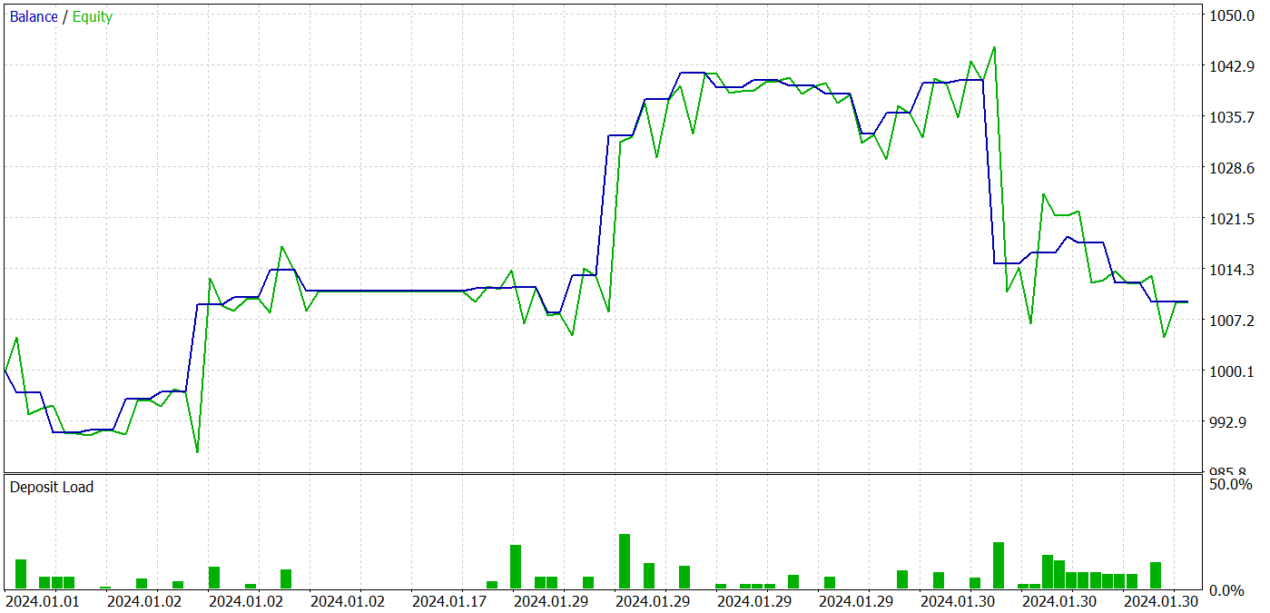
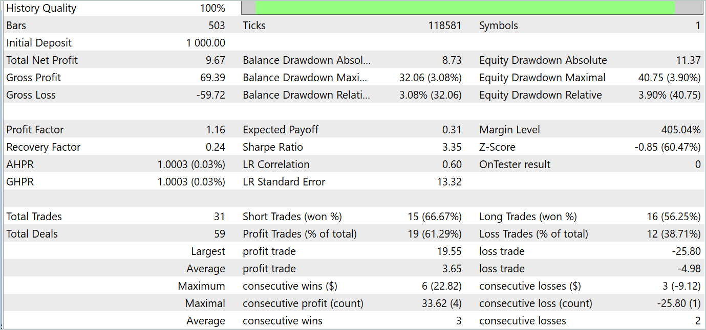
During the testing period, the model made 31 trades, 19 of which were closed with a profit. The share of profitable trades was more than 61%. It is noteworthy that the model had almost an equal number of long and short positions (15 versus 16).
Conclusion
The last two articles were devoted to the ATFNet method which was proposed for forecasting multivariate time series and presented in the paper "ATFNet: Adaptive Time-Frequency Ensembled Network for Long-term Time Series Forecasting". The ATFNet model combines time and frequency domain modules to analyze dependencies in time series data. It uses T-Block to capture local dependencies in the time domain and F-Block to analyze time series cyclicities in the frequency domain.
ATFNet applies dominant harmonic series energy weighting, extended Fourier transform, and complex spectrum attention to adapt to periodicity and frequency offsets in the input time series.
In the practical part of the article, we implemented our vision of the proposed approaches using MQL5. We trained and tested models using real data. The testing results indicate the potential of the proposed approaches for use in constructing profitable trading strategies.
References
- ATFNet: Adaptive Time-Frequency Ensembled Network for Long-term Time Series Forecasting
- Other articles from this series
Programs used in the article
| # | Name | Type | Description |
|---|---|---|---|
| 1 | Research.mq5 | Expert Advisor | Example collection EA |
| 2 | ResearchRealORL.mq5 | Expert Advisor | EA for collecting examples using the Real-ORL method |
| 3 | Study.mq5 | Expert Advisor | Model training EA |
| 4 | StudyEncoder.mq5 | Expert Advisor | Encode Training EA |
| 5 | Test.mq5 | Expert Advisor | Model testing EA |
| 6 | Trajectory.mqh | Class library | System state description structure |
| 7 | NeuroNet.mqh | Class library | A library of classes for creating a neural network |
| 8 | NeuroNet.cl | Code Base | OpenCL program code library |
Translated from Russian by MetaQuotes Ltd.
Original article: https://www.mql5.com/ru/articles/15024
Warning: All rights to these materials are reserved by MetaQuotes Ltd. Copying or reprinting of these materials in whole or in part is prohibited.
This article was written by a user of the site and reflects their personal views. MetaQuotes Ltd is not responsible for the accuracy of the information presented, nor for any consequences resulting from the use of the solutions, strategies or recommendations described.

 Connexus Observer (Part 8): Adding a Request Observer
- Free trading apps
- Over 8,000 signals for copying
- Economic news for exploring financial markets
You agree to website policy and terms of use
Dmitry hello!
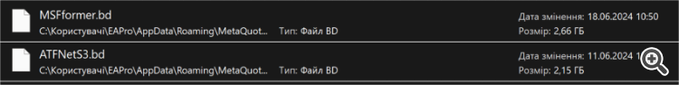
How do you train and replenish the database of examples for a year of history? I have a problem with replenishing new examples in the bd file in your Expert Advisors from the latest articles (where you use a year of history). The thing is that when this file reaches the size of 2 GB, it apparently starts to be saved crookedly and then the model training Expert Advisor can not read it and gives an error. Or the file bd sharply begins to drop in size, with each new addition of examples up to several megabytes and then the training advisor still gives an error. This problem occurs up to 150 trajectories if you take the history for a year and about 250 if you take the history for 7 months. The size of the bd file grows very fast. For example, 18 trajectories weigh almost 500 Mb. 30 trajectories are 700 MB.
As a result, in order to train we have to delete this file with a set of 230 trajectories over 7 months and create it anew with a pre-trained Expert Advisor. But in this mode, the mechanism of updating trajectories when replenishing the database does not work. I assume that this is due to the limitation of 4 GB RAM for one thread in MT5. Somewhere in the help they wrote about it.
What is interesting is that in earlier articles (where the history was for 7 months, and the base for 500 trajectories weighed about 1 GB) such a problem was not present. I am not limited by PC resources as RAM is more than 32 GB and video card memory is enough.
Dmitry, how do you teach with this point in mind or maybe you set up MT5 beforehand?
I use the files from the articles without any modification.
As a result, in order to train we have to delete this file with a set of 230 trajectories over 7 months and create it anew with a pre-trained Expert Advisor. But in this mode, the mechanism of updating trajectories when replenishing the database does not work. I assume that this is due to the limitation of 4 GB RAM for one thread in MT5. It was written about it somewhere in the help.
What is interesting is that in earlier articles (where the history was for 7 months, and the base for 500 trajectories weighed about 1 GB) such a problem was not present. I am not limited by PC resources as RAM is more than 32 GB and the video card has enough memory.
Dmitry, how do you teach with this in mind or maybe you have configured MT5 beforehand?
I use files from articles without any modification.
Victor,
I don't know what to answer you. I work with larger files.
Hi, read this article it's interesting . understand a little, will go trough once again after reading original paper.
I have came across this paper https://www.mdpi.com/2076-3417/14/9/3797#
it claims they archived 94% in bitcoin image classification,is it really possible?