Population optimization algorithms: Changing shape, shifting probability distributions and testing on Smart Cephalopod (SC)

Contents

1. Introduction
2. Test bench for checking distributions
3. Construction of random numbers with the required distribution law
4. Optimization algorithm template - "Smart Cephalopod" algorithm
5. Conclusions

1. Introduction

Probability theory is a mathematical theory that studies random phenomena and determines the likelihood of their occurrence. It allows describing and analyzing random processes. The basic concepts of probability theory are probability, random variable, probability distribution, mathematical expectation and dispersion.

Probability is a numerical characteristic that determines the likelihood of a certain event to occur.

Random variable is a function that associates each outcome of a random experiment with a certain number.

Probability distribution is a function that determines the likelihood of each of the possible values of a random variable.

Mathematical expectation is an average value of a random variable that can be obtained by repeating the experiment many times.

Dispersion is a measure of the distribution of the values of a random variable relative to its mathematical expectation.

Moment is a numerical characteristic of a random variable that describes its distribution. Moments are used to determine the center of a distribution (expectation) and its spread (dispersion and standard deviation), and to analyze the shape of the distribution (skewness and kurtosis). The first moment (n=1) is the mathematical expectation, which determines the center of the random variable distribution. The second point (n=2) is dispersion, which describes the spread of a random variable relative to its mathematical expectation. The third moment (n=3) is a measure of the skewness of the distribution, and the fourth moment (n=4) is a measure of the kurtosis (convexity) of the distribution.

Probability distributions play an important role in modeling random phenomena and data analysis, as well as in statistics for estimating parameters and testing hypotheses. They make it possible to describe the probabilistic properties of random variables and events, as well as determine the probability of various outcomes.

Probability theory and optimization are two important scientific disciplines that are widely used in various fields of science and technology, such as economics, finance, engineering, biology, medicine and many others. The development of these areas and the application of their research and optimization methods makes it possible to solve complex problems and create new technologies, increasing the efficiency and quality of work in various fields including the development of modern technologies for the creation of quantum computers, secure super-fast communications, generative neural networks and artificial intelligence. 

Probabilistic calculations based on probability theory play a key role in modeling random phenomena and analyzing data. Optimization, in turn, is aimed at finding optimal solutions in various problems and allows finding the best solutions among many possible options. However, real world problems feature uncertainty and randomness, and this is where probability distributions come into play. They allow us to take into account randomness and uncertainty in optimization problems.

Probability distributions are also actively used in evolutionary and population algorithms. In these algorithms, the random generation of new states in the search space is modeled using appropriate probability distributions. This allows us to explore the parameter space and find optimal solutions taking into account randomness and diversity in the population.

More sophisticated optimization methods use probability distributions to model uncertainty and approximate complex functions. They allow us to efficiently explore the parameter space and find optimal solutions taking into account randomness and noise in the data.

In this article, we will look at various types of probability distributions, their properties and practical implementation in the form of corresponding functions in code. When generating random numbers with various types of distributions, you can encounter a large number of problems, such as infinite tail lengths or shifting probabilities when setting dispersion boundaries. When designing and creating optimization algorithms, there is often a need to shift probabilities relative to the mathematical expectation. The goal of this article is to solve these problems and create working functions for dealing with probabilities for their subsequent use in optimization algorithms.

2. Test bench for checking distributions

To test and visualize distributions of random variables, we need a test bench that will allow us to clearly display the shape of the distributions. This is important when designing optimization algorithms, since visual representation and understanding of which direction to shift the probability of a random variable helps to achieve the best results.

To build a probability distribution, we need to create something like a series of boxes random numbers will fall into. Boxes are essentially counters. For example, a number line bounded on the left by "min" and on the right by "max" and "in" lying between them can be imagined like this:

min|-----|-----|-----|-----|-----|-----|in|--|--|--|--|--|--|max

We see that the "in" value is shifted on the number line closer to "max". If we generate random numbers in the range [min;max], then the amount of random numbers in the range [min;in] will be greater than in the range [in;max], thereby the probability of numbers falling out will be shifted to the left, creating an imbalance, but we need the number of drops on the left and right to be the same on average, we need to change the shape of the distribution without shifting the probabilities. To do this, the number of boxes to the left and right should be the same (in the schematic example above, this is 6 boxes to the left and right).

So, the test bench for constructing distributions is quite simple. The essence of its work is as follows:

• create a CCanvas object to work with the canvas
• generate a random number with the distribution selected in the settings
• check which area of the corresponding box the random number fell into and add 1 to the box
  
• count the minimum and maximum number of drops among all boxes
• draw circles on the canvas for each box, which corresponds to the amount of random numbers in the boxes
• color the circles in colors from blue (rarely) to red (often)
  

The overall goal of the code is to visualize the probability distribution on the canvas using a graph, where each circle is the amount of random numbers drawn in the boxes, normalized by the min/max number in all boxes.

#property script_show_inputs
#include <Canvas\Canvas.mqh>

enum E_Distribution
{
  uniform = 0,
  gauss   = 1,
  power   = 2,
  levi    = 3
};

//--- input parameters
input double         MinP       = -100.0;
input double         InpP       =  0;
input double         MaxP       =  100.0;
input int            CNT        =  1000000;
input int            Size       =  1000;
input double         SigmaP     =  3;       //Sigma for "Gauss" distribution
input double         PowerP     =  2;       //Power for "Power law" distribution
input double         LeviPowerP =  2;       //Power for "Levy flights" distribution
input E_Distribution Distr_P    = gauss;    //Distribution type

//——————————————————————————————————————————————————————————————————————————————
void OnStart ()
{
  CCanvas Canvas;

  int W = 750;
  int H = 400;
  int O = 10;

  int CountL [];
  int CountR [];

  ArrayResize     (CountL, Size);
  ArrayInitialize (CountL, 0);

  ArrayResize     (CountR, Size);
  ArrayInitialize (CountR, 0);

  string canvasName = "Test_Probability_Distribution_Canvas";
  if (!Canvas.CreateBitmapLabel (canvasName, 5, 30, W, H, COLOR_FORMAT_ARGB_RAW))
  {
    Print ("Error creating Canvas: ", GetLastError ());
    return;
  }

  ObjectSetInteger (0, canvasName, OBJPROP_HIDDEN,     false);
  ObjectSetInteger (0, canvasName, OBJPROP_SELECTABLE, true);

  Canvas.Erase (COLOR2RGB (clrWhite));
  Canvas.Rectangle (1, 1, W - 1, H - 1, COLOR2RGB (clrBlack));

  int    ind = 0;
  double X   = 0.0;

  for (int i = 0; i < CNT; i++)
  {
    switch (Distr_P)
    {
    case uniform:
      X = UniformDistribution (InpP, MinP, MaxP);
      break;
    case gauss:
      X = GaussDistribution (InpP, MinP, MaxP, SigmaP);
      break;
    case power:
      X = PowerDistribution (InpP, MinP, MaxP, PowerP);
      break;
    case levi:
      X = LeviDistribution (InpP, MinP, MaxP, LeviPowerP);
      break;
    }

    if (X < InpP)
    {
      ind = (int)Scale (X, MinP, InpP,
                        0,    Size, false);
      if (ind >= Size) ind = Size - 1;
      if (ind < 0)     ind = 0;
      CountL [ind] += 1;
    }
    else
    {
      ind = (int)Scale (X, InpP, MaxP,
                        0,    Size, false);
      if (ind >= Size) ind = Size - 1;
      if (ind < 0)     ind = 0;
      CountR [ind] += 1;
    }
  }

  int minCNT = CNT;
  int maxCNT = 0;

  for (int i = 0; i < Size; i++)
  {
    if (CountL [i] > maxCNT) maxCNT = CountL [i];
    if (CountR [i] > maxCNT) maxCNT = CountR [i];

    if (CountL [i] < minCNT) minCNT = CountL [i];
    if (CountR [i] < minCNT) minCNT = CountR [i];
  }

  int x = 0.0;
  int y = 0.0;
  color clrF;
  int centre = 0;
  int stepL  = 0;
  int stH_L  = 0;
  int stepR  = 0;
  int stH_R  = 0;

  centre = (int)Scale (InpP, MinP, MaxP, 10, W - 11, false);

  stepL = (centre - O) / Size;
  stH_L = stepL / 2;
  if (stH_L == 0) stH_L = 1;

  stepR = (W - O - centre) / Size;
  stH_R = stepR / 2;
  if (stH_R == 0) stH_R = 1;

  for (int i = 0; i < Size; i++)
  {
    x = (int)Scale (i,          0, Size - 1, O, centre - stH_L, false);
    y = (int)Scale (CountL [i], 0, maxCNT,   O, H - O,  true);

    clrF = DoubleToColor (CountL [i], minCNT, maxCNT, 0, 255);

    Canvas.Circle (x, y, 2, COLOR2RGB (clrF));
    Canvas.Circle (x, y, 3, COLOR2RGB (clrF));


    x = (int)Scale (i,          0, Size - 1, centre + stH_R, W - O, false);
    y = (int)Scale (CountR [i], 0, maxCNT,   O,      H - O, true);

    clrF = DoubleToColor (CountR [i], minCNT, maxCNT, 0, 255);

    Canvas.Circle (x, y, 2, COLOR2RGB (clrF));
    Canvas.Circle (x, y, 3, COLOR2RGB (clrF));
  }

  Canvas.Update ();
}
//——————————————————————————————————————————————————————————————————————————————

3. Construction of random numbers with the required distribution law

Uniform distribution

The uniform distribution is a probability distribution, in which all values of a random variable in a given interval have equal probability. The uniform distribution is widely used to model random variables that are equally likely to take values over a given interval.

Figure 1. Uniform distribution of numbers without a shift

The uniform distribution is the easiest to implement among all. The only point to consider here is that we cannot simply generate numbers in the range [min;max], so we will generate a random number to the left of In or to the right of In depending on the previously generated random number in the range [0.0;1.0]. Therefore, the number of generated numbers on the left and right is equally probable for any position of In relative to [min;max]. There are no problems with out-of-range or artifacts in the distribution.

We can use uniform distribution in all cases when it is necessary to generate a number in a given range with an equal probability of appearing over the entire range.

//——————————————————————————————————————————————————————————————————————————————
double UniformDistribution (const double In, const double outMin, const double outMax)
{
  double rnd = RNDfromCI (0.0, 1.0);

  if (rnd >= 0.5) return RNDfromCI (In, outMax);
  else            return RNDfromCI (outMin, In);
}
//——————————————————————————————————————————————————————————————————————————————

Normal (Gaussian) distribution

The normal distribution is a probability distribution that describes many random phenomena in nature, economics and other fields. It is characterized by a bell shape and symmetry around the average value. The mean and variance of a normal distribution determine it completely.

One of the key properties of the normal distribution is its symmetry around the mean. This means that the probability that a random variable will take a value equal to the mean is greatest, and the probability that it will take a value different from the mean decreases as it moves away from the mean. This property makes the normal distribution especially useful for modeling and data analysis, since it allows us to describe and predict random phenomena that have a mean and deviations from it.

The normal distribution also has many mathematical properties that make it suitable for use in statistical methods and models. For example, if the random variables are independent and have a normal distribution, then their sum will also have a normal distribution. This property allows the normal distribution to be used for modeling and analyzing complex systems consisting of many random variables. The normal distribution has many applications in statistics, physics, economics, finance and other fields. It is the basis for many statistical methods and models, such as linear regression and time series analysis.

For optimization algorithms, the normal distribution is useful in cases where we want to focus attention on a specific location on the number line. In this case, we may only need a part of the curve that forms the distribution form. For example, we want to use a distribution within only three standard deviations. As for anything outside of those boundaries, we cannot just push the values back to the edges of the boundary. If we do this, we will get a frequency of dropouts at the edges that exceeds the frequency at the average value. This problem is demonstrated in Fig. 2. We will solve it in the description below.

To generate a random variable with a normal distribution law, we can use the Box-Muller method.

• First, we need to generate two random uniformly distributed numbers u1 (0, 1] and u2 [0, 1]
• Then we need to calculate the random variable z0 using the equation:

z0 = sqrt(-2 * ln(u1)) * cos(2 * pi * u2)   

• The resulting random variable z0 will have a standard normal distribution
  

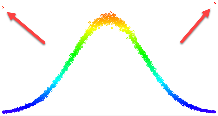
Figure 2. Normal distribution with sigma=3 and artifacts when trying to cut off everything beyond 3 sigmas

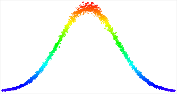
Figure 3. Normal distribution with sigma=3 with a solved problem of artifacts (going beyond the distribution boundaries)

Let's write an implementation of the GaussDistribution function, which generates random values with a normal distribution relative to the "in" average value:

• The following function parameters are set: input value (in), minimum and maximum values of the output range (outMin and outMax) and standard deviation (sigma).
• The natural logarithm of u1 is calculated, which is generated randomly in the range from 0 to 1.
• If u1 is less than or equal to 0, then logN is assigned the value of 0.000000000000001. Otherwise, logN is equal to u1.
• The z0 value is calculated using the normal distribution equation.
• The "sigma" input is checked to see if it is outside the range of the maximum possible standard deviation value equal to 8.583864105157389.
  
• If z0 is greater than or equal to sigmaN, then z0 is assigned a random value in the range from 0 to sigmaN. Otherwise, if z0 is less than or equal to -sigmaN, then z0 is assigned a random value in the range from -sigmaN to 0.0. 
• If z0 is greater than or equal to 0, then the value calculated using the Scale function is returned for the range from 0 to sigmaN and the output range is from "in" to "outMax", otherwise the value calculated using the "Scale" function is returned for the range from -sigmaN to 0 and output range from "outMin" to "in".
  

The point highlighted in yellow is a solution to the problem of the frequency of dropouts at the edges of a given standard deviation. Thus, we simply "spread" the probability that falls outside the boundaries inward to the corresponding part of the distribution curve. In this case, the distribution shape is not violated.

//——————————————————————————————————————————————————————————————————————————————
double C_AO_SC::GaussDistribution (const double In, const double outMin, const double outMax, const double sigma)
{
  double logN = 0.0;
  double u1   = RNDfromCI (0.0, 1.0);
  double u2   = RNDfromCI (0.0, 1.0);

  logN = u1 <= 0.0 ? 0.000000000000001 : u1;

  double z0 = sqrt (-2 * log (logN)) * cos (2 * M_PI * u2);

  double sigmaN = sigma > 8.583864105157389 ? 8.583864105157389 : sigma;

  if (z0 >=  sigmaN) z0 = RNDfromCI (0.0,     sigmaN);
  if (z0 <= -sigmaN) z0 = RNDfromCI (-sigmaN, 0.0);

  if (z0 >= 0.0) z0 =  Scale (z0,        0.0, sigmaN, 0.0, outMax - In, false);
  else           z0 = -Scale (fabs (z0), 0.0, sigmaN, 0.0, In - outMin, false);
  
  return In + z0;
}
//——————————————————————————————————————————————————————————————————————————————

Below is an example of random numbers with a normal distribution (Fig. 4). In this example and below - distributions around the desired value "50" in the range from "-100" to "100" [-100;50;100].

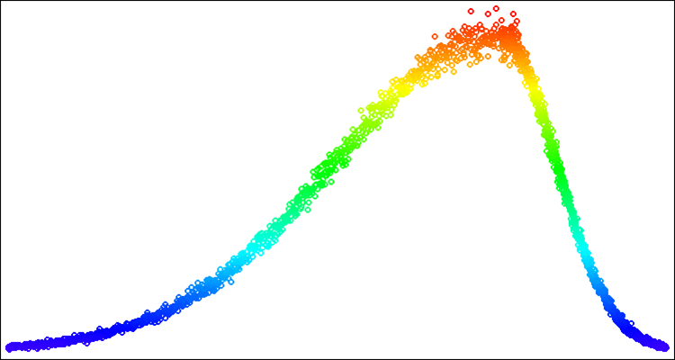
Figure 4. Normal distribution with sigma=3, [-100;50;100]

Power law distribution

The power law distribution is a probability distribution that describes random variables whose probability of taking on very large values decays according to a power law. This distribution is also called Pareto principle or Zipf's law. The power distribution is used in various fields of science and technology. For example, it is used in physics to model the distribution of mass and energy in systems with many particles, such as star clusters and galaxies. It is also used in economics and sociology to analyze the distribution of income and wealth.

The power-law distribution has several interesting properties. First, it is heavy-tailed, which means that the probability that the random variable will take on very large values is not zero. Secondly, it does not have a finite mathematical expectation, which means that the average value of a random variable can be infinite.

The power-law distribution has a very useful form for use in optimization algorithms. It allows concentrating the density of random numbers in places in the search space that require special attention and clarification. However, in its pure form it is unsuitable for use when we want to clearly limit the boundaries of random numbers since it has tails of infinite length, which cannot be "wrapped inward" as easily as in the case of the normal distribution.

For the classical implementation of the power law distribution, it is necessary to use the inverse function. However, in order to get rid of infinity in the tails of the distribution, which interferes with generating values within known limits, we can use a uniformly distributed value raised to a power. Although this is not the correct way to specify a power law distribution, it will allow us to get rid of the infinity in the tails of the distribution while maintaining a distribution shape that is fairly close to the theoretical one. For stochastic optimization algorithms, this is more than sufficient.

The PowerDistribution function takes four double values as inputs: "in", "outMin", "outMax" and "power". It generates a random number "rnd" in the range [-1.0;1.0], calculates the value "r" which is the result of exponentiation of "power", and then scales this value from the range [0.0;1.0] to the given range of values with using the Scale function. If "rnd" is a negative number, then scaling is performed in the range [outMin;in], otherwise - in the range [in;outMax]. The result of the function is returned as a double value.

• If "power" is less than 1, then most of the values in the resulting distribution will be concentrated near zero, and the tail of the distribution will be greatly truncated. This distribution will resemble a parabola.
• If "power" is 1, then the resulting distribution will be uniform.
• If "power" is greater than 1, then most of the values in the resulting distribution will be distributed far from zero, and the tail of the distribution will be long. Such a distribution will have a heavy tail and will resemble the Pareto distribution or power law distribution.
• If "power" tends to infinity, then the resulting distribution will resemble a delta function concentrated at zero.

Thus, a field of additional possibilities opens up for us when using different values of the "power" degree, and therefore we have more opportunities while researching the selection of the optimal distribution to obtain the best result in the optimization algorithm in the context of solving a specific optimization problem.

//——————————————————————————————————————————————————————————————————————————————
double C_AO_SC::PowerDistribution (const double In, const double outMin, const double outMax, const double power)
{
  double rnd = RNDfromCI (-1.0, 1.0);
  double r   = pow (fabs (rnd), power);

  if (rnd >= 0.0) return In + Scale (r, 0.0, 1.0, 0.0, outMax - In, false);
  else            return In - Scale (r, 0.0, 1.0, 0.0, In - outMin, false);
}
//——————————————————————————————————————————————————————————————————————————————

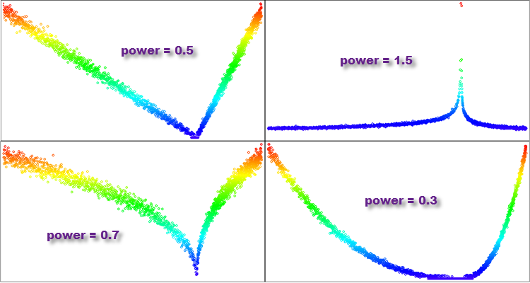
Figure 5. Examples of distributions of the PowerDistribution function with varying degrees of "power"

Levy distribution

Levy's flights are random walks in which the length of each step is determined by the Levy distribution.

The Levy distribution is an example of a distribution with unbounded moments. It describes random variables with heavy tails, which means that the probability of very large values is high. In the Levy distribution, moments may be infinite or non-existent, which makes it special and different from distributions with limited moments, such as the normal distribution.

The heavy tails of the Levy distribution and its unbounded moments make it useful for modeling phenomena that may have extreme values or high variability. Levy's flights have many applications in various fields, including physics, financial mathematics, risk analysis, ecology, economics and engineering. For example, they can be used to model random processes in physics, such as diffusion, turbulence and transport in plasma. They can also be used to model the search strategies of animals and populations, and to optimize parameters in engineering and finance.

The Levy distribution was introduced by French mathematician Paul Lévy in 1925 and has found many applications in various fields of science and technology.

If we are talking about an increment from a specific parameter value in optimization, then in Levy flights each increment is selected from the Levy distribution, and the direction is chosen randomly. This leads to the fact that in Levy flights some steps can be very long, which allows faster exploration of the parameter space than in random walks with a fixed step length (increment).

The form of the Levy flight distribution is similar to the form of the power distribution, but in some cases it is more effective to use one or the other distribution. As in the case of the power law distribution, we will need to get rid of heavy tails. However, in this case, we will do it in a different way, more suitable for this distribution. It was experimentally discovered that it is optimal to use the range [1.0;20.0] for uniformly distributed random numbers involved in generation. We need to calculate the minimum value at the end of the distribution for random numbers to the power of "power", which will serve as our boundary for scaling the generated number into the range [0.0;1.0].

The LeviDistribution function takes four double values as inputs: "in", "outMin", "outMax" and "power", and performs the following steps:

• First of all, the function determines the minimum value "min" based on the "power" parameter. This is the minimum possible function value for subsequent scaling.
  
• Then two random numbers "r1" and "r2" are generated from a uniform distribution on the intervals [0.0;1.0] and [1.0;20.0], respectively.
• The value of "y" is calculated by raising "r2" to the negative power of "power" and scaling it from the interval [min, 1.0] to [0.0;1.0] using the Scale function.
  
• Finally, the function returns the generated value scaled by the [outMin, outMax] interval depending on the value of "r1". If r1 >= 0.5, then the value is scaled by the [in, outMax] interval, otherwise - by the [outMin, in] interval.
  

//——————————————————————————————————————————————————————————————————————————————
double C_AO_SC::LeviDistribution (const double In, const double outMin, const double outMax, const double power)
{
  double min = pow (20.0, -power);
  double r1 = RNDfromCI (0.0, 1.0);
  double r2 = RNDfromCI (1.0, 20.0);
  
  double y = pow (r2, -power);
  y = Scale (y, min, 1.0, 0.0, 1.0, false);
 
  if (r1 >= 0.5) return In + Scale (y, 0.0, 1.0, 0.0, outMax - In, false);
  else           return In - Scale (y, 0.0, 1.0, 0.0, In - outMin, false);
}
//——————————————————————————————————————————————————————————————————————————————

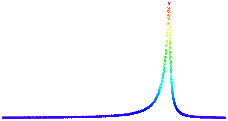
Figure 6. Levy distribution with power = 1.0

4. Optimization algorithm template - "Smart Cephalopod" algorithm

Let's move on to the most interesting stage of our research! Let's check all distributions using an optimization algorithm specially created for these purposes called.... Hmm, what should we call it?

Let's test the idea of such an algorithm: imagine a smart cephalopod that is looking for the most delicious place, so let's assume that its head is in the epicenter of food and is eating something. At the same time, its tentacles constantly spread out to the sides in search of new deposits of food. As soon as one of the tentacles finds a tasty spot, the head moves. Perhaps this is a good idea for an algorithm inspired by sea creatures. Then we know what to call it - it will be Smart Cephalopod!

I am sure this will be an exciting experiment that will allow us to better understand how different distributions work and how they can help us solve complex optimization problems. So let's get started and see what we can find out in this interesting study!

It is logical to set the properties of the cephalopod's legs to the corresponding distribution laws. Then the code for feeling new places with the cephalopod’s feet will look like this:

//----------------------------------------------------------------------------
  for (int i = 0; i < popSize; i++)
  {
    for (int c = 0; c < coords; c++)
    {
      double X   = 0.0;
      double in  = cB [c];
      double min = rangeMin [c];
      double max = rangeMax [c];
      
      switch (distr)
      {
      case uniformDistr: X = UniformDistribution (in, min, max);         break;
      case gaussDistr:   X = GaussDistribution   (in, min, max, powers); break;
      case powerDistr:   X = PowerDistribution   (in, min, max, powers); break;
      case leviDistr:    X = LeviDistribution    (in, min, max, powers); break;
      }

      a [i].c [c] = SeInDiSp  (X, rangeMin [c], rangeMax [c], rangeStep [c]);
    }
  }

This code consists of two nested loops that go through each agent in the "a" array of popSize, and generate a new value for each coordinate element. The generation of a new value is done by selecting one of four types of distributions and applying the appropriate distribution function (UniformDistribution, GaussDistribution, PowerDistribution or LeviDistribution) to the current value of "in" taken from the "cB" array representing the best solution at the moment (where the head is currently located). The resulting new X value is then normalized by the SeInDiSp function using the rangeMin and rangeMax values and the rangeStep for that element. The resulting value is stored in the "a" array for the given agent and coordinate.

Working on this article and specific class methods for generating random numbers with the necessary distributions, convenient for use in building optimization algorithms, led to the understanding that the Rastrigin function has several serious shortcomings that were not obvious at the time of choosing this test function, so I decided not to use it. The good old Rastrigin will be replaced by the Peaks function (a more complete justification will be provided in the next article).

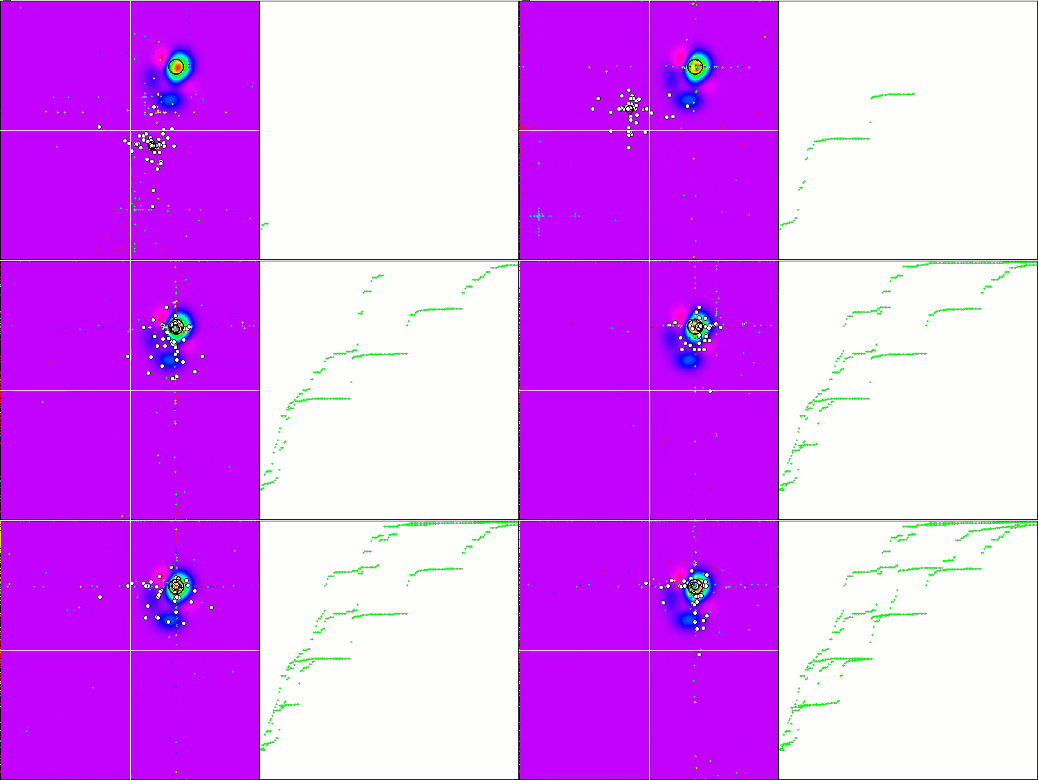
"Smart Cephalopod" in action

5. Summary

To summarize, our experiment with the "Smart Cephalopod" brought interesting results. The animation demonstrates how a random algorithm applying a specific distribution successfully completes a task. I will not reveal exactly what distribution or settings were used, but I will leave it up to you to run your own experiments with the full set of tools in this article. I will be glad if you share your success in the comments.

"Smart Cephalopod" will not be taken into account in the rating table, as it is just an experiment that will help us be more conscious about optimization.

My general conclusions are that the application of a probability distribution and the choice of search strategy play an important role in an optimization problem because it allows one to take into account stochastic factors and more efficiently explore the solution space and discover areas with a high probability of finding the best solutions.

However, just using the probability distribution is not sufficient. It is also important to consider the choice and features of the search strategy. Different search strategies may have advantages and disadvantages depending on the optimization problem.

Therefore, in order to achieve even better results when designing optimization algorithms both in a specific problem and in general, it is necessary to use the probability distribution and the search strategy selection together. These elements should work in tandem to provide the required performance of the developed optimization algorithm. Overall, the results of this experiment highlight the importance of taking a deliberate approach to optimization. For example, applying probability distributions and choosing an appropriate search strategy can be useful in the field of machine learning, where optimization and finding optimal solutions are required.

One of the important features of the tools presented in this article is the possibility of shifting distributions in a given range of values. You will not find distribution shifting capabilities in specialized libraries that focus on general problems. This allows researchers to manipulate and tune probability distributions according to the required characteristics of the optimization algorithm. Adjusting and controlling the probability bias together with elements of the search strategy can really work wonders!