
Neural networks made easy (Part 65): Distance Weighted Supervised Learning (DWSL)

Introduction
Behavior cloning methods, largely based on the principles of supervised learning, show fairly good results. But their main problem remains the search for ideal role models, which are sometimes very difficult to collect. In turn, reinforcement learning methods are able to work with non-optimal raw data. At the same time, they can find suboptimal policies to achieve the goal. However, when searching for an optimal policy, we often encounter an optimization problem that is more relevant in high-dimensional and stochastic environments.
To bridge the gap between these two approaches, a group of scientists proposed the Distance Weighted Supervised Learning (DWSL) method and presented it in the article "Distance Weighted Supervised Learning for Offline Interaction Data". It is an offline supervised learning algorithm for goal-conditioned policy. Theoretically, DWSL converges to an optimal policy with a minimum return boundary at the level of trajectories from the training set. The practical examples in the article demonstrate the superiority of the proposed method over imitation learning and reinforcement learning algorithms. I suggest taking a closer look at this DWSL algorithm. We will evaluate its strengths and weaknesses in solving our practical problems.
1. DWSL algorithm
Authors of the Distance Weighted Supervised Learning method set the goal of obtaining an algorithm capable of using the largest possible set of data for training. In this paradigm, they assume that the Agent acts in a deterministic Markov Decision Process with:
- state space S;
- action space A;
- deterministic dynamics St+1 = F(St,At), where St+1 is the resulting new state from taking the action At at state St;
- goal space G;
- sparse goal-conditioned reward function R(S,A,G);
- discount factor γ.
The goal space G is a subspace of the state space S with a goal extraction function G = φ(St), which is often identical to φ(St) = St+n. The objective of the algorithm is to learn a goal-conditioned policy π(A|S,G), which has mastery over the studied environment and is able to reach the set goal and then remain at it. To obtain the desired result, we maximize the discounted return from the reward function R(S,A,G) subject to achieving the goal G from the target distribution p(G).
While this problem setup differs from those discussed earlier, it has strong connections with two general problem settings: the Stochastic Shortest Path problem and GCRL.
The authors of the method note that works in the field of GCRL assume the presence of trajectories with labeled subgoals. These subgoals are specified by the policy intent, which provides the model with information about the distribution of goals p(G) during testing. This limits the data from which the offline GCRL can learn. The reason is that many offline data sources do not contain goal labels (subgoals) along with each trajectory. Moreover, goals can be difficult to obtain.
In order to learn from the broadest set of offline data, the authors of the method consider a more general situation. The situation does not involve access to true environmental dynamics, reward labels, or the test-time goal distribution. At the training stage, only a set of trajectories from states and actions of an arbitrary level of optimality is used. Distribution p(G) is taken to be the distribution of goals induced by applying the goal extraction function φ(St) over all states in the dataset. It is assumed that for most practical datasets, the goals around the data distribution are likely to be close to the goals for tasks problems of interest. The DWSL method can use any sparse reward function that can be computed purely from existing state-action sequences. However, in practice, the method authors found empirical estimation also worked quite well.
Intuitively, the best goal-achieving strategy when using the specified reward function to reach goal G from the current state S is to use the path with the minimum number of time steps (shortest path). However, the trajectories in the training dataset do not necessarily follow the shortest paths. As a result, behavior cloning techniques may exhibit suboptimal behavior.
To address this problem, DWSL estimates distances using supervised learning, evaluating the trained models within the distribution of the training dataset. The model learns the entire distribution of pairwise distances between states in the training dataset. It then uses this distribution to estimate the minimum distance to the target contained in each state's dataset. After that, it learns the policy to follow these paths. Below is the visualization of the DWSL method provided by the authors.
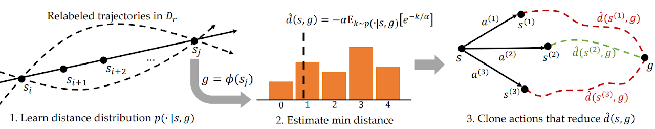
Between any two states Si and Sj on the same trajectory, for i < j there is at least one path of "j - i" time steps. Using this property, we generate a labeled dataset that contains all pairwise distances between states and targets in the training dataset. For each State-Goal pair sampled from the new distribution, we model a discrete distribution over the number of time steps k from the current state to the goal, as shown in Figure 1 on the left. This allows us to obtain a parameterized estimate of this distribution via maximum likelihood under the labeled dataset:
![]()
In practice, the distribution is modeled as a discrete classifier over possible distances. The shortest path between the source and goal states contained within the labeled dataset is determined by the minimum number of time steps k. However, because the distribution is learned using function approximation, estimating the minimum distance in this manner will likely exploit modeling errors. To minimize this error, the authors of the method propose to compute LogSumExp over the distribution to obtain a soft estimate of the minimum distance:
![]()
Note that in the formula presented, the distance is multiplied by "-1" to obtain the minimum estimate instead of the maximum. Here α is the temperature hyperparameter. When α tends to "0", the value of the function d(s, g) approaches the minimum distance k.
After learning minimum distance estimates, we want to follow the known paths that originate from each state. Assume that the Agent is in state S and needs to achieve goal G. In the initial state, the Agent can perform one of two actions (A1 or A2), which lead to states S1 and S2, respectively. We prefer to take the first action if it is the beginning of a path to the goal with a minimum number of steps (smaller estimated distance to the goal). Therefore, we want to weigh the likelihood of different actions by their estimates of distance to the target (right in the Figure above). However, naively weighting actions this way would result in a larger weighting for all data points close to the goal, since any state far from the goal will naturally have a larger distance. Instead, we weigh the likelihood of actions according to their reduction in the estimated distance to the target, which the method authors refer to as the Advantage. This allows us to formulate a new goal for training the model:
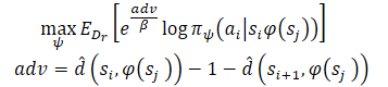
The authors of the method use exponentiated Advantages to ensure that all weights are positive.
2. Implementation using MQL5
After getting acquainted with the theoretical aspects of the Distance Weighted Supervised Learning method, we can move on to the practical part of our article, in which we will create a version of the method implementation in MQL5. As always, we will try to combine the proposed algorithm with the knowledge we have previously accumulated. We will also try to reproduce our perception of the proposed approaches. I agree that this approach to some extent distances us from the authors' algorithm and is not its exact reproduction. Consequently, all weaknesses that can be identified during testing relate only to this implementation.
The original s article presents experiments on controlling robotics applications. In such conditions, goal setting plays a dominant role in achieving a positive result. Moreover, the goal is clear in every individual case. In my implementation, I focus on maximizing the robot's profitability during the training period. To simplify the model, I decided not to set a subgoal at each step. Which in turn allows us not to train a goal setting model.
Here we will train the model using Actor-Critic approaches. For the donor, we will use the model of Stochastic Marginal Actor-Critic (SMAC). We will supplement it with other developments. In particular, we will add a mechanism for weighing trajectories from CWBC. But first things first. We begin our work by describing the architecture of the models.
2.1. Model architecture
As always, the architecture of the trained models is represented in the CreateDescriptions method. In parameters, we will pass to the method pointers to dynamic arrays of architecture descriptions of 3 models:
- Actor
- Critic
- Random encoder
I should remind you here that the SMAC algorithm provides for training a stochastic latent state encoder, which we previously included in the Actor architecture with the ability to be used by the Critic. We will use this solution in this implementation.
In the body of the method, we check the received pointers and, if necessary, create new object instances.
bool CreateDescriptions(CArrayObj *actor, CArrayObj *critic, CArrayObj *convolution)
  {
//---
   CLayerDescription *descr;
//---
   if(!actor)
     {
      actor = new CArrayObj();
      if(!actor)
         return false;
     }
   if(!critic)
     {
      critic = new CArrayObj();
      if(!critic)
         return false;
     }
   if(!convolution)
     {
      convolution = new CArrayObj();
      if(!convolution)
         return false;
     }
We input into the Actor historical data of price movement and indicator values, which is reflected in the size of its raw data layer.
//--- Actor
   actor.Clear();
//--- Input layer
   if(!(descr = new CLayerDescription()))
      return false;
   descr.type = defNeuronBaseOCL;
   int prev_count = descr.count = (HistoryBars * BarDescr);
   descr.activation = None;
   descr.optimization = ADAM;
   if(!actor.Add(descr))
     {
      delete descr;
      return false;
     }
We feed into the model raw unprocessed data. Therefore, after the raw data layer, we use a batch data normalization layer. It brings the raw data obtained from various sources into a comparable form.
//--- layer 1
   if(!(descr = new CLayerDescription()))
      return false;
   descr.type = defNeuronBatchNormOCL;
   descr.count = prev_count;
   descr.batch = 1000;
   descr.activation = None;
   descr.optimization = ADAM;
   if(!actor.Add(descr))
     {
      delete descr;
      return false;
     }
After that we try to identify stable data patterns using convolutional layers. To obtain a probabilistic representation of the assignment of source data to stable patterns, we use the SoftMax function.
//--- layer 2
   if(!(descr = new CLayerDescription()))
      return false;
   descr.type = defNeuronConvOCL;
   prev_count = descr.count = HistoryBars;
   descr.window = BarDescr;
   descr.step = BarDescr;
   int prev_wout = descr.window_out = BarDescr / 2;
   descr.activation = LReLU;
   descr.optimization = ADAM;
   if(!actor.Add(descr))
     {
      delete descr;
      return false;
     }
//--- layer 3
   if(!(descr = new CLayerDescription()))
      return false;
   descr.type = defNeuronSoftMaxOCL;
   descr.count = prev_count;
   descr.step = prev_wout;
   descr.optimization = ADAM;
   descr.activation = None;
   if(!convolution.Add(descr))
     {
      delete descr;
      return false;
     }
//--- layer 4
   if(!(descr = new CLayerDescription()))
      return false;
   descr.type = defNeuronConvOCL;
   prev_count = descr.count = prev_count;
   descr.window = prev_wout;
   descr.step = prev_wout;
   prev_wout = descr.window_out = 8;
   descr.activation = LReLU;
   descr.optimization = ADAM;
   if(!actor.Add(descr))
     {
      delete descr;
      return false;
     }
//--- layer 5
   if(!(descr = new CLayerDescription()))
      return false;
   descr.type = defNeuronSoftMaxOCL;
   descr.count = prev_count;
   descr.step = prev_wout;
   descr.optimization = ADAM;
   descr.activation = None;
   if(!convolution.Add(descr))
     {
      delete descr;
      return false;
     }
Please note that we search for stable patterns in the context of each individual candlestick of historical data.
The pattern search results are analyzed by two fully connected layers.
//--- layer 6
   if(!(descr = new CLayerDescription()))
      return false;
   descr.type = defNeuronBaseOCL;
   descr.count = LatentCount;
   descr.optimization = ADAM;
   descr.activation = LReLU;
   if(!actor.Add(descr))
     {
      delete descr;
      return false;
     }
//--- layer 7
   if(!(descr = new CLayerDescription()))
      return false;
   descr.type = defNeuronBaseOCL;
   prev_count = descr.count = LatentCount;
   descr.activation = LReLU;
   descr.optimization = ADAM;
   if(!actor.Add(descr))
     {
      delete descr;
      return false;
     }
To the obtained data, we add a description of the account status.
//--- layer 8
   if(!(descr = new CLayerDescription()))
      return false;
   descr.type = defNeuronConcatenate;
   descr.count = 2 * LatentCount;
   descr.window = prev_count;
   descr.step = AccountDescr;
   descr.optimization = ADAM;
   descr.activation = SIGMOID;
   if(!actor.Add(descr))
     {
      delete descr;
      return false;
     }
Then generate the stochastic latent state provided by the SMAC method.
//--- layer 9
   if(!(descr = new CLayerDescription()))
      return false;
   descr.type = defNeuronVAEOCL;
   descr.count = LatentCount;
   descr.optimization = ADAM;
   if(!actor.Add(descr))
     {
      delete descr;
      return false;
     }
Next comes a decision-making block of 2 fully connected layers.
//--- layer 10
   if(!(descr = new CLayerDescription()))
      return false;
   descr.type = defNeuronBaseOCL;
   descr.count = LatentCount;
   descr.activation = LReLU;
   descr.optimization = ADAM;
   if(!actor.Add(descr))
     {
      delete descr;
      return false;
     }
//--- layer 11
   if(!(descr = new CLayerDescription()))
      return false;
   descr.type = defNeuronBaseOCL;
   descr.count = LatentCount;
   descr.activation = LReLU;
   descr.optimization = ADAM;
   if(!actor.Add(descr))
     {
      delete descr;
      return false;
     }
At the Actor output, we set a variational autoencoder block to make the policy stochastic. The size of the results layer corresponds to the dimension of the Agent's action vector.
//--- layer 12
   if(!(descr = new CLayerDescription()))
      return false;
   descr.type = defNeuronBaseOCL;
   descr.count = 2 * NActions;
   descr.activation = SIGMOID;
   descr.optimization = ADAM;
   if(!actor.Add(descr))
     {
      delete descr;
      return false;
     }
//--- layer 13
   if(!(descr = new CLayerDescription()))
      return false;
   descr.type = defNeuronVAEOCL;
   descr.count = NActions;
   descr.optimization = ADAM;
   if(!actor.Add(descr))
     {
      delete descr;
      return false;
     }
The Critic architecture is used unchanged. The input of the model is a latent representation of the environment state from the Actor's hidden layer. The data obtained does not require conversion into a comparable form. Therefore, we will not use a batch normalization layer in this model.
//--- Critic
   critic.Clear();
//--- Input layer
   if(!(descr = new CLayerDescription()))
      return false;
   descr.type = defNeuronBaseOCL;
   prev_count = descr.count = LatentCount;
   descr.activation = None;
   descr.optimization = ADAM;
   if(!critic.Add(descr))
     {
      delete descr;
      return false;
     }
To the latent representation, we add the actions of the Actor.
//--- layer 1
   if(!(descr = new CLayerDescription()))
      return false;
   descr.type = defNeuronConcatenate;
   descr.count = LatentCount;
   descr.window = prev_count;
   descr.step = NActions;
   descr.optimization = ADAM;
   descr.activation = LReLU;
   if(!critic.Add(descr))
     {
      delete descr;
      return false;
     }
The concatenated data is analyzed by a decision-making block of 3 fully connected layers. The size of the last layer corresponds to the size of the decomposed reward vector.
//--- layer 2
   if(!(descr = new CLayerDescription()))
      return false;
   descr.type = defNeuronBaseOCL;
   descr.count = LatentCount;
   descr.activation = LReLU;
   descr.optimization = ADAM;
   if(!critic.Add(descr))
     {
      delete descr;
      return false;
     }
//--- layer 3
   if(!(descr = new CLayerDescription()))
      return false;
   descr.type = defNeuronBaseOCL;
   descr.count = LatentCount;
   descr.activation = LReLU;
   descr.optimization = ADAM;
   if(!critic.Add(descr))
     {
      delete descr;
      return false;
     }
//--- layer 4
   if(!(descr = new CLayerDescription()))
      return false;
   descr.type = defNeuronBaseOCL;
   descr.count = NRewards;
   descr.optimization = ADAM;
   descr.activation = None;
   if(!critic.Add(descr))
     {
      delete descr;
      return false;
     }
At the end of the CreateDescriptions method, we add a description of the random Encoder architecture. Looking ahead a little, I will say that we will use the Encoder as part of the process for determining the distance between environmental states. To describe a single state of the environment, we use 2 vectors:
- of historical price and indicator data
- of account status and open positions
We will feed the concatenated vector of these two entities into the Encoder.
//--- Convolution
   convolution.Clear();
//--- Input layer
   if(!(descr = new CLayerDescription()))
      return false;
   descr.type = defNeuronBaseOCL;
   prev_count = descr.count = (HistoryBars * BarDescr) + AccountDescr;
   descr.activation = None;
   descr.optimization = ADAM;
   if(!convolution.Add(descr))
     {
      delete descr;
      return false;
     }
The Encoder model is not trained. Therefore, the use of a batch normalization layer will not give the required result. Therefore, to bring the data into some comparable form, we will use a fully connected layer. Then we will normalize the data using the SoftMax layer.
//--- layer 1
   if(!(descr = new CLayerDescription()))
      return false;
   descr.type = defNeuronBaseOCL;
   descr.count = HistoryBars * BarDescr;
   descr.optimization = ADAM;
   descr.activation = None;
   if(!convolution.Add(descr))
     {
      delete descr;
      return false;
     }
//--- layer 2
   if(!(descr = new CLayerDescription()))
      return false;
   descr.type = defNeuronSoftMaxOCL;
   descr.count = HistoryBars;
   descr.step = BarDescr;
   descr.optimization = ADAM;
   descr.activation = None;
   if(!convolution.Add(descr))
     {
      delete descr;
      return false;
     }
Next comes a block of convolutional layers, which is also covered with a SoftMax layer.
//--- layer 3
   if(!(descr = new CLayerDescription()))
      return false;
   descr.type = defNeuronConvOCL;
   prev_count = descr.count = HistoryBars;
   descr.window = BarDescr;
   descr.step = BarDescr;
   prev_wout = descr.window_out = BarDescr / 2;
   descr.activation = LReLU;
   descr.optimization = ADAM;
   if(!convolution.Add(descr))
     {
      delete descr;
      return false;
     }
//--- layer 4
   if(!(descr = new CLayerDescription()))
      return false;
   descr.type = defNeuronConvOCL;
   prev_count = descr.count = prev_count;
   descr.window = prev_wout;
   descr.step = prev_wout;
   prev_wout = descr.window_out = prev_wout / 2;
   descr.activation = LReLU;
   descr.optimization = ADAM;
   if(!convolution.Add(descr))
     {
      delete descr;
      return false;
     }
//--- layer 5
   if(!(descr = new CLayerDescription()))
      return false;
   descr.type = defNeuronConvOCL;
   prev_count = descr.count = prev_count;
   descr.window = prev_wout;
   descr.step = prev_wout;
   prev_wout = descr.window_out = 2;
   descr.activation = LReLU;
   descr.optimization = ADAM;
   if(!convolution.Add(descr))
     {
      delete descr;
      return false;
     }
//--- layer 6
   if(!(descr = new CLayerDescription()))
      return false;
   descr.type = defNeuronSoftMaxOCL;
   descr.count = prev_count * prev_wout;
   descr.optimization = ADAM;
   descr.activation = None;
   if(!convolution.Add(descr))
     {
      delete descr;
      return false;
     }
At the output of the Encoder, we use a fully connected layer, which returns the embedding of the analyzed state of the environment.
//--- layer 7
   if(!(descr = new CLayerDescription()))
      return false;
   descr.type = defNeuronBaseOCL;
   descr.count = EmbeddingSize;
   descr.activation = LReLU;
   descr.optimization = ADAM;
   if(!convolution.Add(descr))
     {
      delete descr;
      return false;
     }
//---
   return true;
  }
2.2 Preparing helper methods
After describing the architecture of the models used, we move on to working on the implementation of the model training algorithm. But before implementing the learning process, let's discuss the methods that implement individual blocks of the general algorithm.
First, we will use the weighting and prioritization of trajectories, which was discussed within the framework of the CWBC method. For this, we will migrate the GetProbTrajectories and SampleTrajectory methods. Their algorithm was described in detail in the previous article, so we will not dwell on it now.
To train the Actor and Critics, we will use rewards and actions weighted using DWSL method approaches. In order to eliminate repeated operations, we will combine the calculation of target vectors for both models within one GetTargets method. To enable the possibility to transfer 2 vectors within one operation, we will create a structure.
struct STarget
  {
   vector<float>     rewards;
   vector<float>     actions;
  };
Thus, the GetTargets method receives in parameters:
- percentile for determining the number of closest analyzed states from the training set;
- embedding of the analyzed state;
- matrix of state embeddings in the training set;
- matrix of rewards from the training set;
- matrix of Agent actions from the training set.
The last 3 matrices correspond to each other.
Based on the results of the work, the method returns the structure of their 2 target vectors.
STarget GetTargets(int percentile,
                   vector<float> &embedding,
                   matrix<float> &state_embedding,
                   matrix<float> &rewards,
                   matrix<float> &actions
                  )
  {
   STarget result;
In the method body, we declare the structure of the results and immediately check the correspondence of the embedding sizes of the analyzed state and in the matrix of states from the training set.
   if(embedding.Size() != state_embedding.Cols())
     {
      PrintFormat("%s -> %d Inconsistent embedding size", __FUNCTION__, __LINE__);
      return result;
     }
Next, we determine the distance between the analyzed state and the states from the training set. To determine the soft distance, we use LogSumExp proposed by the authors of the DWSL method.
   ulong size = embedding.Size();
   ulong states = state_embedding.Rows();
   ulong k = ulong(states * percentile / 100);
   matrix<float> temp = matrix<float>::Zeros(states, size);
   for(ulong i = 0; i < size; i++)
      temp.Col(MathAbs(state_embedding.Col(i) - embedding[i]), i);
   float alpha=temp.Max();
   vector<float> dist = MathLog(MathExp(temp/(-alpha)).Sum(1))*(-alpha);
After that we create local matrices of rewards, actions and embedding. Data about the closest states will be transferred to that matrices.
   vector<float> min_dist = vector<float>::Zeros(k);
   matrix<float> k_rewards = matrix<float>::Zeros(k, NRewards);
   matrix<float> k_actions = matrix<float>::Zeros(k, NActions);
   matrix<float> k_embedding = matrix<float>::Zeros(k + 1, size);
   matrix<float> U, V;
   vector<float> S;
   float max = dist.Percentile(percentile);
   float min = dist.Min();
   for(ulong i = 0, cur = 0; (i < states && cur < k); i++)
     {
      if(max < dist[i])
         continue;
      min_dist[cur] = dist[i];
      k_rewards.Row(rewards.Row(i), cur);
      k_actions.Row(actions.Row(i), cur);
      k_embedding.Row(state_embedding.Row(i), cur);
      cur++;
     }
   k_embedding.Row(embedding, k);
To obtain the target reward vector for training, we need to weigh the matrix of selected rewards based on the distance from the analyzed state. Note that the minimum distance will give us the minimum weight of the corresponding reward. However, this contradicts the general logic: the most relevant value has minimal impact on the final result. This can be easily fixed. We will simply multiply the distance vector by "-1". The SoftMax function will transform the obtained values into the probability plane. Now we just need to multiply the resulting probability vector by the collected reward matrix of the closest states.
   vector<float> sf;
   (min_dist*(-1)).Activation(sf, AF_SOFTMAX);
   result.rewards = sf.MatMul(k_rewards);
Here we also add nuclear norms to encourage the Actor to learn.
   k_embedding.SVD(U, V, S);
   result.rewards[NRewards - 2] = S.Sum() / (MathSqrt(MathPow(k_embedding, 2.0f).Sum() * MathMax(k + 1, size)));
   result.rewards[NRewards - 1] = EntropyLatentState(Actor);
Next, we form a target vector of actions. This time we will weigh actions by their preferential reward. Similar to the distance vector, we will calculate the reward vector using the LogSumExp function.
   vector<float> act_sf;
   alpha=MathAbs(k_rewards).Max();
   dist = MathLog(MathExp(k_rewards/(-alpha)).Sum(1))*(-alpha);
This time the maximum reward should have the maximum impact, so we don't need to reverse the values. We simply transfer rewards to the area of probabilistic values using the SoftMax function. After that, we multiply the resulting vector by the action matrix. The result is written into the structure. Then we return both vectors of target values to the caller.
With this we complete the preparatory work and move on to the implementation of the main algorithm.
2.3 Training data collection Expert Advisor
Next, we move on to a data collection program for offline model training. As before, this task will be implemented in the Expert Advisor "...\DWSL\Research.mq5". We will not fully review the entire code of this EA, as most of its methods have been used and considered in detail in earlier articles. Let's look at the key features. Let's start with the OnTick tick handling method, the body of which implements the main algorithm.
At the beginning of the method, we check if a new bar has opened and, if necessary, load historical price and indicator data.
void OnTick()
  {
//---
   if(!IsNewBar())
      return;
//---
   int bars = CopyRates(Symb.Name(), TimeFrame, iTime(Symb.Name(), TimeFrame, 1), HistoryBars, Rates);
   if(!ArraySetAsSeries(Rates, true))
      return;
//---
   RSI.Refresh();
   CCI.Refresh();
   ATR.Refresh();
   MACD.Refresh();
   Symb.Refresh();
   Symb.RefreshRates();
Using the obtained data, we form a buffer of initial data.
   float atr = 0;
   for(int b = 0; b < (int)HistoryBars; b++)
     {
      float open = (float)Rates[b].open;
      float rsi = (float)RSI.Main(b);
      float cci = (float)CCI.Main(b);
      atr = (float)ATR.Main(b);
      float macd = (float)MACD.Main(b);
      float sign = (float)MACD.Signal(b);
      if(rsi == EMPTY_VALUE || cci == EMPTY_VALUE || atr == EMPTY_VALUE || macd == EMPTY_VALUE || sign == EMPTY_VALUE)
         continue;
      //---
      int shift = b * BarDescr;
      sState.state[shift] = (float)(Rates[b].close - open);
      sState.state[shift + 1] = (float)(Rates[b].high - open);
      sState.state[shift + 2] = (float)(Rates[b].low - open);
      sState.state[shift + 3] = (float)(Rates[b].tick_volume / 1000.0f);
      sState.state[shift + 4] = rsi;
      sState.state[shift + 5] = cci;
      sState.state[shift + 6] = atr;
      sState.state[shift + 7] = macd;
      sState.state[shift + 8] = sign;
     }
   bState.AssignArray(sState.state);
And an account status buffer.
   sState.account[0] = (float)AccountInfoDouble(ACCOUNT_BALANCE);
   sState.account[1] = (float)AccountInfoDouble(ACCOUNT_EQUITY);
//---
   double buy_value = 0, sell_value = 0, buy_profit = 0, sell_profit = 0;
   double position_discount = 0;
   double multiplyer = 1.0 / (60.0 * 60.0 * 10.0);
   int total = PositionsTotal();
   datetime current = TimeCurrent();
   for(int i = 0; i < total; i++)
     {
      if(PositionGetSymbol(i) != Symb.Name())
         continue;
      double profit = PositionGetDouble(POSITION_PROFIT);
      switch((int)PositionGetInteger(POSITION_TYPE))
        {
         case POSITION_TYPE_BUY:
            buy_value += PositionGetDouble(POSITION_VOLUME);
            buy_profit += profit;
            break;
         case POSITION_TYPE_SELL:
            sell_value += PositionGetDouble(POSITION_VOLUME);
            sell_profit += profit;
            break;
        }
      position_discount += profit - (current - PositionGetInteger(POSITION_TIME)) * multiplyer * MathAbs(profit);
     }
   sState.account[2] = (float)buy_value;
   sState.account[3] = (float)sell_value;
   sState.account[4] = (float)buy_profit;
   sState.account[5] = (float)sell_profit;
   sState.account[6] = (float)position_discount;
   sState.account[7] = (float)Rates[0].time;
//---
   bAccount.Clear();
   bAccount.Add((float)((sState.account[0] - PrevBalance) / PrevBalance));
   bAccount.Add((float)(sState.account[1] / PrevBalance));
   bAccount.Add((float)((sState.account[1] - PrevEquity) / PrevEquity));
   bAccount.Add(sState.account[2]);
   bAccount.Add(sState.account[3]);
   bAccount.Add((float)(sState.account[4] / PrevBalance));
   bAccount.Add((float)(sState.account[5] / PrevBalance));
   bAccount.Add((float)(sState.account[6] / PrevBalance));
   double x = (double)Rates[0].time / (double)(D'2024.01.01' - D'2023.01.01');
   bAccount.Add((float)MathSin(2.0 * M_PI * x));
   x = (double)Rates[0].time / (double)PeriodSeconds(PERIOD_MN1);
   bAccount.Add((float)MathCos(2.0 * M_PI * x));
   x = (double)Rates[0].time / (double)PeriodSeconds(PERIOD_W1);
   bAccount.Add((float)MathSin(2.0 * M_PI * x));
   x = (double)Rates[0].time / (double)PeriodSeconds(PERIOD_D1);
   bAccount.Add((float)MathSin(2.0 * M_PI * x));
We transfer the collected data to the Actor model and call the feed-forward method. Remember to control the execution of operations.
   if(bAccount.GetIndex() >= 0)
      if(!bAccount.BufferWrite())
         return;
//---
   if(!Actor.feedForward(GetPointer(bState), 1, false, GetPointer(bAccount)))
      return;
As a result of the feed-forward pass, the Actor model generates an action vector, which we decrypt. Here we only remove the volume of counter operations, which does not generate profit. Unlike other previously discussed works, we do not add noise to the resulting vector to explore the environment. The stochastic policy of the Actor, together with the stochasticity of the latent state, already generates a sufficient spread of actions to explore the immediate environment of the action space.
   PrevBalance = sState.account[0];
   PrevEquity = sState.account[1];
//---
   vector<float> temp;
   Actor.getResults(temp);
//---
   double min_lot = Symb.LotsMin();
   double step_lot = Symb.LotsStep();
   double stops = MathMax(Symb.StopsLevel(), 1) * Symb.Point();
   if(temp[0] >= temp[3])
     {
      temp[0] -= temp[3];
      temp[3] = 0;
     }
   else
     {
      temp[3] -= temp[0];
      temp[0] = 0;
     }
Next, we compare the existing position with the Actor's forecast and, if necessary, perform trading operations. First for long positions.
//--- buy control
   if(temp[0] < min_lot || (temp[1] * MaxTP * Symb.Point()) <= stops || (temp[2] * MaxSL * Symb.Point()) <= stops)
     {
      if(buy_value > 0)
         CloseByDirection(POSITION_TYPE_BUY);
     }
   else
     {
      double buy_lot = min_lot + MathRound((double)(temp[0] - min_lot) / step_lot) * step_lot;
      double buy_tp = NormalizeDouble(Symb.Ask() + temp[1] * MaxTP * Symb.Point(), Symb.Digits());
      double buy_sl = NormalizeDouble(Symb.Ask() - temp[2] * MaxSL * Symb.Point(), Symb.Digits());
      if(buy_value > 0)
         TrailPosition(POSITION_TYPE_BUY, buy_sl, buy_tp);
      if(buy_value != buy_lot)
        {
         if(buy_value > buy_lot)
            ClosePartial(POSITION_TYPE_BUY, buy_value - buy_lot);
         else
            Trade.Buy(buy_lot - buy_value, Symb.Name(), Symb.Ask(), buy_sl, buy_tp);
        }
     }
Then repeat for short positions.
//--- sell control
   if(temp[3] < min_lot || (temp[4] * MaxTP * Symb.Point()) <= stops || (temp[5] * MaxSL * Symb.Point()) <= stops)
     {
      if(sell_value > 0)
         CloseByDirection(POSITION_TYPE_SELL);
     }
   else
     {
      double sell_lot = min_lot + MathRound((double)(temp[3] - min_lot) / step_lot) * step_lot;;
      double sell_tp = NormalizeDouble(Symb.Bid() - temp[4] * MaxTP * Symb.Point(), Symb.Digits());
      double sell_sl = NormalizeDouble(Symb.Bid() + temp[5] * MaxSL * Symb.Point(), Symb.Digits());
      if(sell_value > 0)
         TrailPosition(POSITION_TYPE_SELL, sell_sl, sell_tp);
      if(sell_value != sell_lot)
        {
         if(sell_value > sell_lot)
            ClosePartial(POSITION_TYPE_SELL, sell_value - sell_lot);
         else
            Trade.Sell(sell_lot - sell_value, Symb.Name(), Symb.Bid(), sell_sl, sell_tp);
        }
     }
At the end of the method operations, all need to collect feedback from the environment and transfer the data to the experience replay buffer.
   sState.rewards[0] = bAccount[0];
   sState.rewards[1] = 1.0f - bAccount[1];
   if((buy_value + sell_value) == 0)
      sState.rewards[2] -= (float)(atr / PrevBalance);
   else
      sState.rewards[2] = 0;
   for(ulong i = 0; i < NActions; i++)
      sState.action[i] = temp[i];
   sState.rewards[3] = 0;
   sState.rewards[4] = 0;
   if(!Base.Add(sState))
      ExpertRemove();
  }
At this point, the data collection process can be considered completed. But the work on this Expert Advisor has not yet been completed. As part of the implementation of the DWSL method, I would like to draw your attention to one detail. In the theoretical part of this article, we have mentioned that the DWSL method converges to the optimal policy with a minimum return boundary at the level of trajectories from the training set. Naturally, in searching for the optimal trajectory, we would like to raise the minimum profitability limit as high as possible. To this end, we will make changes to the process of adding new trajectories to the experience replay buffer. After the initial filling of the buffer, we will gradually replace passes with minimal profitability with more profitable ones. This process is implemented in the OnTesterPass method, which processes the pass completion event in the strategy tester.
In the method body, we first initialize local variables. Immediately create a loop to poll pass frames.
void OnTesterPass()
  {
//---
   ulong pass;
   string name;
   long id;
   double value;
   STrajectory array[];
   while(FrameNext(pass, name, id, value, array))
     {
In the body of the loop, we check whether the frame matches the current program.
      int total = ArraySize(Buffer);
      if(name != MQLInfoString(MQL_PROGRAM_NAME))
         continue;
      if(id <= 0)
         continue;
After that, the process branches out depending on how the experience replay buffer is filled. If the buffer is already filled to the maximum specified size, then we search the buffer for a pass with the lowest return. This could be the highest loss or the lowest profit.
      if(total >= MaxReplayBuffer)
        {
         for(int a = 0; a < id; a++)
           {
            float min = FLT_MAX;
            int min_tr = 0;
            for(int i = 0; i < total; i++)
              {
               float prof = Buffer[i].States[Buffer[i].Total - 1].account[1];
               if(prof < min)
                 {
                  min = MathMin(prof, min);
                  min_tr = i;
                 }
              }
Next, we compare the resulting value with the return of the last pass. If it is higher, write the data of the new pass instead of the lowest found return. Otherwise, move on to the next pass.
            float prof = array[a].States[array[a].Total - 1].account[1];
            if(min <= prof)
              {
               Buffer[min_tr] = array[a];
               PrintFormat("Replace %.2f to %.2f -> bars %d", min, prof, array[a].Total);
              }
           }
        }
If the buffer is not yet full, simply add a new pass without unnecessary control operations.
      else
        {
         if(ArrayResize(Buffer, total + (int)id, 10) < 0)
            return;
         ArrayCopy(Buffer, array, total, 0, (int)id);
        }
     }
  }
We operate the following priority:
- Maximum filling of the experience replay buffer to provide trained models with the most complete information about the environment.
- After filling the experience replay buffer, select the most profitable passes to build an optimal strategy.
The complete code of the Expert Advisor and all its methods are presented in the attachment. The attachments also include the code of the model testing Expert Advisor "...\DWSL\Test.mq5". It has a similar algorithm to the tick processing method but is intended for a single run in the strategy tester. We will not consider it within the scope of this article.
2.4 Model training EA
The model training process is implemented in the Expert Advisor "...\DWSL\Study.mq5". We will not discuss in detail all its methods. Let's only see the Train method, which organizes the main algorithm for training the models.
In the body of the method, we define the size of the experience replay buffer and save it in a local tick counter state variable to track the time spent on operations.
void Train(void)
  {
   int total_tr = ArraySize(Buffer);
   uint ticks = GetTickCount();
Next, we loop through all trajectories to count the total number of states in the experience replay buffer. This will enable us to prepare matrices of sufficient size to record state embeddings, as well as the corresponding rewards and actions of the Agent. We have already seen the use of these matrices in the GetTargets method.
   int total_states = Buffer[0].Total;
   for(int i = 1; i < total_tr; i++)
      total_states += Buffer[i].Total;
   vector<float> temp, next;
   Convolution.getResults(temp);
   matrix<float> state_embedding = matrix<float>::Zeros(total_states, temp.Size());
   matrix<float> rewards = matrix<float>::Zeros(total_states, NRewards);
   matrix<float> actions = matrix<float>::Zeros(total_states, NActions);
The next step is to fill out these matrices. To do this, we create a system of loops with a complete search of all states from the experience replay buffer. In the body of this loop system, we collect a description of each individual state into a single data buffer.
   int state = 0;
   for(int tr = 0; tr < total_tr; tr++)
     {
      for(int st = 0; st < Buffer[tr].Total; st++)
        {
         State.AssignArray(Buffer[tr].States[st].state);
         float PrevBalance = Buffer[tr].States[MathMax(st - 1, 0)].account[0];
         float PrevEquity = Buffer[tr].States[MathMax(st - 1, 0)].account[1];
         State.Add((Buffer[tr].States[st].account[0] - PrevBalance) / PrevBalance);
         State.Add(Buffer[tr].States[st].account[1] / PrevBalance);
         State.Add((Buffer[tr].States[st].account[1] - PrevEquity) / PrevEquity);
         State.Add(Buffer[tr].States[st].account[2]);
         State.Add(Buffer[tr].States[st].account[3]);
         State.Add(Buffer[tr].States[st].account[4] / PrevBalance);
         State.Add(Buffer[tr].States[st].account[5] / PrevBalance);
         State.Add(Buffer[tr].States[st].account[6] / PrevBalance);
         double x = (double)Buffer[tr].States[st].account[7] / (double)(D'2024.01.01' - D'2023.01.01');
         State.Add((float)MathSin(x != 0 ? 2.0 * M_PI * x : 0));
         x = (double)Buffer[tr].States[st].account[7] / (double)PeriodSeconds(PERIOD_MN1);
         State.Add((float)MathCos(x != 0 ? 2.0 * M_PI * x : 0));
         x = (double)Buffer[tr].States[st].account[7] / (double)PeriodSeconds(PERIOD_W1);
         State.Add((float)MathSin(x != 0 ? 2.0 * M_PI * x : 0));
         x = (double)Buffer[tr].States[st].account[7] / (double)PeriodSeconds(PERIOD_D1);
         State.Add((float)MathSin(x != 0 ? 2.0 * M_PI * x : 0));
Then, in the feed-forward pass of the encoder, we generate its embedding.
         if(!Convolution.feedForward(GetPointer(State), 1, false, NULL))
           {
            PrintFormat("%s -> %d", __FUNCTION__, __LINE__);
            ExpertRemove();
            return;
           }
         Convolution.getResults(temp);
The output vector is saved in the state_embedding matrix.
         if(!state_embedding.Row(temp, state))
            continue;
The relevant data from the experience replay buffer is saved in the 'rewards' and Agent's 'actions' matrices.
         if(!temp.Assign(Buffer[tr].States[st].rewards) ||
            !next.Assign(Buffer[tr].States[st + 1].rewards) ||
            !rewards.Row(temp - next * DiscFactor, state))
            continue;
         if(!temp.Assign(Buffer[tr].States[st].action) ||
            !actions.Row(temp, state))
            continue;
Please note that we only add Benefits for moving to the next state to the reward matrix. In addition, if any error occurs, we do not completely terminate the program, but just move on to the next state. Thus, we do not complete the entire learning process, but only slightly reduce the base for comparison.
Then we increment the counter of saved embeddings. Before moving on to the next iteration of our loop system, we inform the user about the progress of the state encoding process.
         state++;
         if(GetTickCount() - ticks > 500)
           {
            string str = StringFormat("%-15s %6.2f%%", "Embedding ", state * 100.0 / (double)(total_states));
            Comment(str);
            ticks = GetTickCount();
           }
        }
     }
Once the encoding process is complete, we reduce our matrices to the actual amount of data populated.
   if(state != total_states)
     {
      rewards.Resize(state, NRewards);
      actions.Resize(state, NActions);
      state_embedding.Reshape(state, state_embedding.Cols());
      total_states = state;
     }
The next step is to prepare local variables and organize the prioritizing of trajectories. The process of computing the probabilities of choosing trajectories is implemented in a separate GetProbTrajectories method, the algorithm of which was presented in the previous article.
   vector<float> rewards1, rewards2, target_reward;
   STarget target;
//---
   vector<float> probability = GetProbTrajectories(Buffer, 0.9);
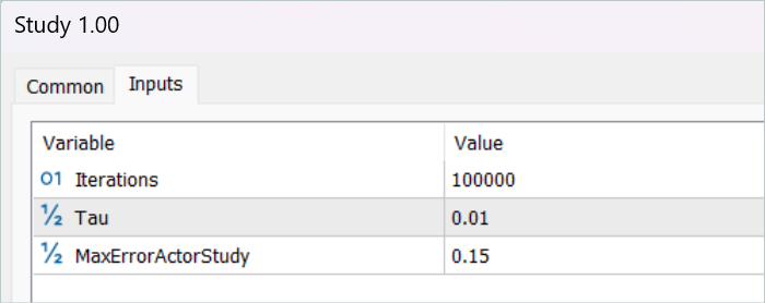
This completes the data preparation stage. Next, we move on to the model training algorithm, which is also organized in a loop. The number of iterations of the model training loop is indicated in the external parameters of the Expert Advisor.
In the loop body, we first sample the trajectory taking into account the probabilities computed above. The process is implemented in the SampleTrajectory method; its algorithm was also presented in the previous article. Then we sample the state on the selected trajectory.
   vector<float> probability = GetProbTrajectories(Buffer, 0.9);
   int bar = (HistoryBars - 1) * BarDescr;
   for(int iter = 0; (iter < Iterations && !IsStopped()); iter ++)
     {
      int tr = SampleTrajectory(probability);
      int i = (int)((MathRand() * MathRand() / MathPow(32767, 2)) * (Buffer[tr].Total - 2));
      if(i < 0)
        {
         iter--;
         continue;
        }
Next, I organized the branching process depending on the completed training iterations. I exclude the estimation of the subsequent state by the target models at the initial stage since the estimation of states by untrained models is completely random and can lead the learning process in the wrong direction. In turn, the assessment of the subsequent state by models with a sufficient level of accuracy will allow us to estimate the expected future return from the policy used at this step. Thereby, we can prioritize actions taking into account subsequent returns.
In this block, we fill the initial data buffer with a description of the subsequent state of the environment.
         State.AssignArray(Buffer[tr].States[i + 1].state);
         float PrevBalance = Buffer[tr].States[i].account[0];
         float PrevEquity = Buffer[tr].States[i].account[1];
         Account.Clear();
         Account.Add((Buffer[tr].States[i + 1].account[0] - PrevBalance) / PrevBalance);
         Account.Add(Buffer[tr].States[i + 1].account[1] / PrevBalance);
         Account.Add((Buffer[tr].States[i + 1].account[1] - PrevEquity) / PrevEquity);
         Account.Add(Buffer[tr].States[i + 1].account[2]);
         Account.Add(Buffer[tr].States[i + 1].account[3]);
         Account.Add(Buffer[tr].States[i + 1].account[4] / PrevBalance);
         Account.Add(Buffer[tr].States[i + 1].account[5] / PrevBalance);
         Account.Add(Buffer[tr].States[i + 1].account[6] / PrevBalance);
         double x = (double)Buffer[tr].States[i + 1].account[7] / (double)(D'2024.01.01' - D'2023.01.01');
         Account.Add((float)MathSin(x != 0 ? 2.0 * M_PI * x : 0));
         x = (double)Buffer[tr].States[i + 1].account[7] / (double)PeriodSeconds(PERIOD_MN1);
         Account.Add((float)MathCos(x != 0 ? 2.0 * M_PI * x : 0));
         x = (double)Buffer[tr].States[i + 1].account[7] / (double)PeriodSeconds(PERIOD_W1);
         Account.Add((float)MathSin(x != 0 ? 2.0 * M_PI * x : 0));
         x = (double)Buffer[tr].States[i + 1].account[7] / (double)PeriodSeconds(PERIOD_D1);
         Account.Add((float)MathSin(x != 0 ? 2.0 * M_PI * x : 0));
Generate Agent actions taking into account the updated policy.
         if(Account.GetIndex() >= 0)
            Account.BufferWrite();
         if(!Actor.feedForward(GetPointer(State), 1, false, GetPointer(Account)))
           {
            PrintFormat("%s -> %d", __FUNCTION__, __LINE__);
            break;
           }
Then, evaluate the resulting action with two models of target Critics.
         if(!TargetCritic1.feedForward(GetPointer(Actor), LatentLayer, GetPointer(Actor)) ||
            !TargetCritic2.feedForward(GetPointer(Actor), LatentLayer, GetPointer(Actor)))
           {
            PrintFormat("%s -> %d", __FUNCTION__, __LINE__);
            break;
           }
We use the minimum estimate to calculate the expected reward.
         TargetCritic1.getResults(rewards1);
         TargetCritic2.getResults(rewards2);
         target_reward.Assign(Buffer[tr].States[i + 1].rewards);
         if(rewards1.Sum() <= rewards2.Sum())
            target_reward = rewards1 - target_reward;
         else
            target_reward = rewards2 - target_reward;
         target_reward[NRewards - 1] = EntropyLatentState(Actor);
         target_reward *= DiscFactor;
        }
At the next stage, we move on to the process of training Critic models. These models are trained using states and actions from the experience replay buffer.
First, we copy the descriptions of the current state of the environment into the source data buffer.
      //--- Q-function study
      State.AssignArray(Buffer[tr].States[i].state);
Then we create a buffer for describing the account status.
      float PrevBalance = Buffer[tr].States[MathMax(i - 1, 0)].account[0];
      float PrevEquity = Buffer[tr].States[MathMax(i - 1, 0)].account[1];
      Account.Clear();
      Account.Add((Buffer[tr].States[i].account[0] - PrevBalance) / PrevBalance);
      Account.Add(Buffer[tr].States[i].account[1] / PrevBalance);
      Account.Add((Buffer[tr].States[i].account[1] - PrevEquity) / PrevEquity);
      Account.Add(Buffer[tr].States[i].account[2]);
      Account.Add(Buffer[tr].States[i].account[3]);
      Account.Add(Buffer[tr].States[i].account[4] / PrevBalance);
      Account.Add(Buffer[tr].States[i].account[5] / PrevBalance);
      Account.Add(Buffer[tr].States[i].account[6] / PrevBalance);
      double x = (double)Buffer[tr].States[i].account[7] / (double)(D'2024.01.01' - D'2023.01.01');
      Account.Add((float)MathSin(x != 0 ? 2.0 * M_PI * x : 0));
      x = (double)Buffer[tr].States[i].account[7] / (double)PeriodSeconds(PERIOD_MN1);
      Account.Add((float)MathCos(x != 0 ? 2.0 * M_PI * x : 0));
      x = (double)Buffer[tr].States[i].account[7] / (double)PeriodSeconds(PERIOD_W1);
      Account.Add((float)MathSin(x != 0 ? 2.0 * M_PI * x : 0));
      x = (double)Buffer[tr].States[i].account[7] / (double)PeriodSeconds(PERIOD_D1);
      Account.Add((float)MathSin(x != 0 ? 2.0 * M_PI * x : 0));
      if(Account.GetIndex() >= 0)
         Account.BufferWrite();
The collected data allows us to run a feed-forward pass of the Actor.
      if(!Actor.feedForward(GetPointer(State), 1, false, GetPointer(Account)))
        {
         PrintFormat("%s -> %d", __FUNCTION__, __LINE__);
         break;
        }
Please note that we run the feed-forward Actor pass before training Critics. Although during the training process we will use actions from the experience replay buffer. This is due to the use of the Actor's latent state as the Critics' input.
Next, we fill the action buffer from the training database and call the feed-forward pass methods of our Critics.
      Actions.AssignArray(Buffer[tr].States[i].action);
      if(Actions.GetIndex() >= 0)
         Actions.BufferWrite();
      //---
      if(!Critic1.feedForward(GetPointer(Actor), LatentLayer, GetPointer(Actions)) ||
         !Critic2.feedForward(GetPointer(Actor), LatentLayer, GetPointer(Actions)))
        {
         PrintFormat("%s -> %d", __FUNCTION__, __LINE__);
         break;
        }
We will use weighted rewards as target values for training models. To obtain them, we first add a description of the account state to the buffer of the current state of the environment and generate an embedding of the analyzed state.
      if(!State.AddArray(GetPointer(Account)) || !Convolution.feedForward(GetPointer(State), 1, false, NULL))
        {
         PrintFormat("%s -> %d", __FUNCTION__, __LINE__);
         break;
        }
      Convolution.getResults(temp);
The dataset available at this stage is enough to call the previously discussed GetTargets method, which will return the vectors of weighted rewards and actions.
target = GetTargets(Percent, temp, state_embedding, rewards, actions);
With the target data in hand, we can run the backpropagation pass of the Critic models. But first we correct the error gradient using the CAGrad method.
      Critic1.getResults(rewards1);
      Result.AssignArray(CAGrad(target.rewards + target_reward - rewards1) + rewards1);
      if(!Critic1.backProp(Result, GetPointer(Actions), GetPointer(Gradient)) ||
         !Actor.backPropGradient(GetPointer(Account), GetPointer(Gradient), LatentLayer))
        {
         PrintFormat("%s -> %d", __FUNCTION__, __LINE__);
         break;
        }

      Critic2.getResults(rewards2);
      Result.AssignArray(CAGrad(target.rewards + target_reward - rewards2) + rewards2);
      if(!Critic2.backProp(Result, GetPointer(Actions), GetPointer(Gradient)) ||
         !Actor.backPropGradient(GetPointer(Account), GetPointer(Gradient), LatentLayer))
        {
         PrintFormat("%s -> %d", __FUNCTION__, __LINE__);
         break;
        }
In the next step, we update the Actor's policy. We have already run the feed-forward pass of the model earlier. Also, we have obtained a weighted vector of target actions. Therefore, we have all the necessary data to perform a backpropagation pass in the supervised learning mode.
      //--- Policy study
      Actor.getResults(rewards1);
      Result.AssignArray(CAGrad(target.actions - rewards1) + rewards1);
      if(!Actor.backProp(Result, GetPointer(Account), GetPointer(Gradient)))
        {
         PrintFormat("%s -> %d", __FUNCTION__, __LINE__);
         break;
        }
As you can see, when forming the vector of target actions of the Actor, we used the Advantages of actions extracted directly from the experience replay buffer. Therefore, trained Critic models were not used. Please note that regardless of the Actor's policy, its influence on market movements is minimal. Thus, overestimating the Advantage using an approximated Critic can distort the data by modeling error. In such a paradigm, training Critic models may seem unnecessary. But we still want to take into account the impact of the studied policies on expected future returns. For this purpose, we select the Critic that demonstrates the lowest error as a result of training. We also evaluate the Actor's actions generated by the new policy. The gradient of the deviation of the resulting estimate from the weighted one is then passed to the Actor to optimize the parameters.
      CNet *critic = NULL;
      if(Critic1.getRecentAverageError() <= Critic2.getRecentAverageError())
         critic = GetPointer(Critic1);
      else
         critic = GetPointer(Critic2);
      if(MathAbs(critic.getRecentAverageError()) <= MaxErrorActorStudy)
        {
         if(!critic.feedForward(GetPointer(Actor), LatentLayer, GetPointer(Actor)))
           {
            PrintFormat("%s -> %d", __FUNCTION__, __LINE__);
            break;
           }
         critic.getResults(rewards1);
         Result.AssignArray(CAGrad(target.rewards + target_reward - rewards1) + rewards1);
         critic.TrainMode(false);
         if(!critic.backProp(Result, GetPointer(Actor)) ||
            !Actor.backPropGradient(GetPointer(Account), GetPointer(Gradient)))
           {
            PrintFormat("%s -> %d", __FUNCTION__, __LINE__);
            critic.TrainMode(true);
            break;
           }
         critic.TrainMode(true);
        }
Note that these operations are performed only if we are confident enough that the Critic will provide an adequate assessment of the actions. To regulate this process, we have introduced an additional external parameter MaxErrorActorStudy, which determines the maximum error of the Critic's assessment for enabling the specified process.
After completing the model training process, we copy the parameters of the trained Critic models to the target models. It should also be noted here that at the initial stage, before enabling the process of assessing subsequent states, we transfer the parameters of the trained models to the target ones in full. The use of the mechanism for estimating subsequent states enables soft copying of parameters.
      //--- Update Target Nets
      if(iter >= StartTargetIter)
        {
         TargetCritic1.WeightsUpdate(GetPointer(Critic1), Tau);
         TargetCritic2.WeightsUpdate(GetPointer(Critic2), Tau);
        }
      else
        {
         TargetCritic1.WeightsUpdate(GetPointer(Critic1), 1);
         TargetCritic2.WeightsUpdate(GetPointer(Critic2), 1);
        }
This completes the operations of one model training iteration. Now we only need to inform the user about the progress of the model training process and move on to the next iteration.
      if(GetTickCount() - ticks > 500)
        {
         string str = StringFormat("%-15s %5.2f%% -> Error %15.8f\n", "Critic1", iter * 100.0 / (double)(Iterations),
                                                                                    Critic1.getRecentAverageError());
         str += StringFormat("%-15s %5.2f%% -> Error %15.8f\n", "Critic2", iter * 100.0 / (double)(Iterations),
                                                                                    Critic2.getRecentAverageError());
         str += StringFormat("%-14s %5.2f%% -> Error %15.8f\n", "Actor", iter * 100.0 / (double)(Iterations),
                                                                                      Actor.getRecentAverageError());
         Comment(str);
         ticks = GetTickCount();
        }
     }
After successfully completing all iterations of the model training cycle, we clear the comments field on the chart. Inform the user about the learning outcomes and initiate the Expert Advisor termination.
   Comment("");
//---
   PrintFormat("%s -> %d -> %-15s %10.7f", __FUNCTION__, __LINE__, "Critic1", Critic1.getRecentAverageError());
   PrintFormat("%s -> %d -> %-15s %10.7f", __FUNCTION__, __LINE__, "Critic2", Critic2.getRecentAverageError());
   PrintFormat("%s -> %d -> %-15s %10.7f", __FUNCTION__, __LINE__, "Actor", Actor.getRecentAverageError());
   ExpertRemove();
//---
  }
This concludes the practical part of our article. Find the complete code of all programs used in the article in the attachment. We move on to the testing phase.
3. Testing
We have done extensive work to implement our vision of the DWSL method using MQL5. I must admit that we ended up with a kind of conglomerate from a number of previously discussed methods. This is quite a big experiment. The effectiveness of our solution can be checked on historical data. This is what we will do now.
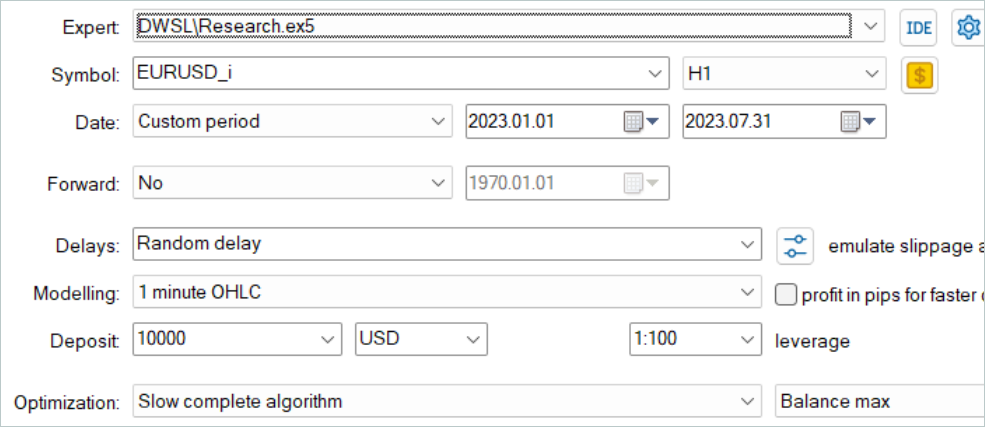
As in all previous cases, model training is carried out using the EURUSD H1 data for the first 7 months of 2023. Data for training models was collected out in the MetaTrader 5 strategy tester in the full parameter optimization mode. In the first stage, we collect 500 random trajectories. Since we have optimized the OnTesterPass method algorithm, we can run a little more passes. Those showing the best returns will be selected for the experience replay buffer.
Please note here that we should not strive to obtain profitable passages of random policies. It is a rather random process at this stage. As we have seen earlier, the probability of obtaining a completely profitable pass by a random policy over the entire interval is close to 0. Fortunately, the DWSL method is capable of working with raw data of any quality.
After collecting the training dataset, we run our model training Expert Advisor for the first time.
At this stage, I have not achieved a completely profitable strategy. This is largely attributable to the low returns of passes from the training dataset. But it should be noted that re-running the Expert Advisor that interacts with the environment, after the first training cycle, gave trajectories with noticeably higher returns. There was one, possibly random, profit-making run during the entire training period. This generally demonstrates the effectiveness of the method and promises the possibility of achieving better results.
After several iterations of collecting trajectories and training, I managed to get a model that could consistently generate profits. The resulting model was tested using historical data of August 2023, which was not included in the training set. However, since they directly followed the training period, we can assume that the datasets were comparable.


According to the testing results, the model managed to make a profit, reaching a profit factor of 1.3. The balance graph shows quite a rapid growth in the first half of the month. Then it had fluctuations in a rather narrow range. The following testing results can be considered positive:
- More than 50% of positions are profitable.
- The maximum profitable trade is almost 4 times the maximum losing one, and the average profitable trade is almost a quarter greater than the average losing one.
- There are trades in both directions (60% short and 40% long). Almost 55% of short and 46% of long positions were closed with a profit.
- The longest profitable series exceeds the longest losing series both in the number of trades and in amount.
The results obtained generally create a positive impression.
Conclusion
In this article, we introduced another interesting method for training models, Distance Weighted Supervised Learning. By using a weighted assessment of available data, it allows the offline optimization of collected non-optimal trajectories and training of quite interesting policies. They subsequently demonstrate good results.
The effectiveness of the considered method is confirmed by our practical results. During the training process, we have obtained a policy that was capable of generalizing the learned material to new data. As a result, we got a profitable balance graph during testing.
However, once again, I would like to remind you that all the programs presented in the article are intended only to demonstrate the technology and are not ready for use in real trading.
References
Programs used in the article
| # | Name | Type | Description |
|---|---|---|---|
| 1 | Research.mq5 | EA | Example collection EA |
| 2 | Study.mq5 | EA | Agent training EA |
| 3 | Test.mq5 | EA | Model testing EA |
| 4 | Trajectory.mqh | Class library | System state description structure |
| 5 | NeuroNet.mqh | Class library | A library of classes for creating a neural network |
| 6 | NeuroNet.cl | Code Base | OpenCL program code library |
Translated from Russian by MetaQuotes Ltd.
Original article: https://www.mql5.com/ru/articles/13779
Warning: All rights to these materials are reserved by MetaQuotes Ltd. Copying or reprinting of these materials in whole or in part is prohibited.
This article was written by a user of the site and reflects their personal views. MetaQuotes Ltd is not responsible for the accuracy of the information presented, nor for any consequences resulting from the use of the solutions, strategies or recommendations described.

- Free trading apps
- Over 8,000 signals for copying
- Economic news for exploring financial markets
You agree to website policy and terms of use