
Neural networks made easy (Part 64): ConserWeightive Behavioral Cloning (CWBC) method

Introduction
The Decision Transformer and all its modifications, which we discussed in recent articles, belong to the methods of Behavior Cloning (BC). We train models to repeat actions from "expert" trajectories depending on the state of the environment and the target outcomes. Thus, we teach the model to imitate the behavior of an expert in the current state of the environment in order to achieve the target.
However, in real conditions, different expert assessments of the same state of the environment differ quite greatly. Sometimes they are completely opposite. Moreover, I want to remind you that in previous works we did not involve experts to create our training set. We used various methods for sampling the Agent's actions and selected the best trajectories. These trajectories were not always optimal.
In the process of sampling trajectories in a continuous space of actions and episodes, it is almost impossible to save all possible options. Only a small part of the sampled trajectories can at least partially satisfy our requirements. Such trajectories are more like outliers that the model can simply discard during the training process.
To combat this situation, we used the approaches of the Go-Explore method. Then, using small pieces, we successively formed a successful trajectory. Such trajectories can be called suboptimal. They are close to our expectations, but their optimality remains unproven.
O course, we can mark the optimal trajectory using historical data manually. This approach brings us closer to supervised learning with all the pros and cons of this approach.
At the same time, selecting optimal passes puts the model in ideal conditions, which can lead to model overfitting. In this case the model, having learned the route of the training sample, cannot generalize the experience gained to new environmental states.
The second problematic aspect of behavior cloning methods is setting goals for the model (Return To Go, RTG). We have already discussed this issue in previous works. Some works recommend using the coefficient to the maximum result from the training set, which often produces better results. But this approach is applicable only for solving static problems. Such a coefficient is selected for each task separately. The Dichotomy of Control method offers another solution to this problem. There are other approaches as well.
The problems voiced above are addressed by the authors of the article "Reliable Conditioning of Behavioral Cloning for Offline Reinforcement Learning". To solve these problems, the authors propose a rather interesting method, ConserWeightive Behavioral Cloning (CWBC), which is applicable not only to models of the Decision Transformer family.
1. The Algorithm
In order to identify factors influencing the reliability of reinforcement learning methods that depend on target rewards, the authors of the article Reliable Conditioning of Behavioral Cloning for Offline Reinforcement Learning designed two illustrative experiments.
In the first experiment, they run models of different architectures on datasets of trajectories with different levels of returns, from almost random to expert and suboptimal. The results of the experiment demonstrated that the reliability of the model largely depends on the quality of the training dataset. When training models on data from average and expert return trajectories, the model demonstrates reliable results under the condition of high RTG. At the same time, when training a model on low-scoring trajectories, its performance quickly decreases after a certain point in which RTG increases. This is because low-quality data does not provide enough information to train policies that are conditional on large rewards. This has a negative effect on the reliability of the resulting model.
Data quality is not the only reason for the model's reliability. The model architecture also plays an important role. In the experiments conducted, DT shows reliability in all three datasets. It is assumed that DT reliability is achieved by using a Transformer architecture. Since the Agent's next action prediction policy is based on a sequence of environmental states and RTG labels, attention layers can ignore RTG labels outside the training dataset distribution. This also shows good forecasting accuracy. At the same time, models built on the MLP architecture, receiving the current state and RTG as input data for generating actions, cannot ignore information about the desired reward. To test this hypothesis, the authors experiment with a slightly modified version of DT in which the environmental and RTG vectors are concatenated at each time step. Thus, the model cannot ignore the RTG information in the sequence. The experimental results demonstrate a rapid decrease in the reliability of such a model after the RTG leaves the distribution of the training set. Which confirms the assumption made above.
To optimize the model training process and minimize the influence of the above factors, the article authors suggest the use of the ConserWeightive Behavioral Cloning (CWBC) framework, which is a fairly simple yet effective way to improve the reliability of existing methods to train behavior cloning models. CWBC consists of two components:
- Trajectory weighing
- Conservative RTG regularization
Trajectory weighting provides a systematic way to transform suboptimal data distributions to more accurately estimate the optimal distribution by increasing the weight of high-return trajectories. The conservative loss regularizer encourages the policy to remain close to the original data distribution, subject to large targets.
1.1 Trajectory weighting
We know that the optimal offline distribution of trajectories is simply the distribution of demonstrations generated by the optimal policy. Typically, the offline distribution of trajectories will be biased relative to the optimal one. During training, this leads to a gap between training and testing, since we want to condition our Agent to maximize its return when evaluating and operating the model, but are forced to minimize the empirical risk on a biased data distribution during training.
The main idea of the method is to transform the training sample of trajectories into a new distribution that better estimates the optimal trajectory. The new distribution should focus on high-return trajectories, which intuitively mitigates the train-test gap. Since we expect the original dataset to contain very few high-return trajectories, a mere elimination of low-return trajectories will eliminate the majority of training data. This will lead to poor data efficiency. The method authors propose to weight the trajectories based on their returns.
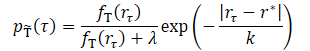
where λ, k are two hyperparameters that determine the shape of the transformed distribution.
The smoothing parameter k controls how trajectories are weighted based on their returns. Intuitively, smaller k gives more weight to high-return trajectories. As the parameter value increases, the transformed distribution becomes more uniform. The authors propose setting the k value as the difference between the maximum and the z-th percentile value of the results in the training dataset.
![]()
This allows the actual value of k to adapt to different datasets. The method authors tested four z values from the set {99, 90, 50, 0}, which correspond to four increasing k values. According to the experimental results for each dataset, the transformed distribution using small k is highly concentrated on high rewards. As k increases, the density of low-return trajectories increases and the distribution becomes more uniform. With relatively small values of k based on the percentile from the set {99, 90, 50}, the model demonstrates good performance on all datasets. However, large values of k based on percentile 0 degrade performance for the expert trajectory dataset.
The parameter λ also affects the transformed distribution. When λ = 0, the transformed distribution concentrates on high returns. As λ increases, the transformed distribution tends to the original, but is still weighted toward the high-return region due to the influence of the exponential term. The actual performance of the models with different values of λ shows similar results that are better or comparable to training on the original dataset.
1.2 Conservative regularization
As mentioned above, the architecture also plays an important role in the reliability of the trained model. The idealized scenario is hard or even impossible to achieve. But the authors of the CWBC method require a model to at least stay close to the original data distribution in order to avoid a catastrophic failure when specifying an RTG outside the distribution. In other words, the policy must be conservative. However, conservatism does not necessarily have to come from the architecture, but can also arise from a proper model training loss function, as is typically done in conservative methods based on state and transition cost estimation.
The authors of the method propose a new conservative regularizer for return-conditioned behavioral cloning methods that explicitly encourage the policy to stay close to the original data distribution. The idea is to enforce the predicted actions when conditioning on large out-of-distribution returns to stay close to in-distribution actions. This is achieved by adding positive noise to RTGs for trajectories with high return and penalize the L2 distance between the predicted action and the ground truth. To guarantee that large returns are generated outside the distribution, we generate noise such that the adjusted RTG value is no less than the highest return in the training set.
The authors propose to apply conservative regularization to trajectories whose returns exceed the qth percentile of rewards in the training set. This ensures that when specifying an RTG outside of the training distribution, the policy behaves similarly to high-return trajectories rather than a random trajectory. We add noise and offset the RTG at each time step.
The experiments conducted by the method authors demonstrate that using the 95th percentile generally works well in a variety of environments and data sets.
The authors of the method note that the proposed conservative regularizer differs from other conservative components for offline RL methods based on estimating the costs of states and transitions. While the latter typically attempt to adjust the estimation of the cost function to prevent extrapolation error, the proposed method distorts the return-to-go to create out-of-distribution conditions and adjusts the prediction of actions.
By using trajectory weighting together with a conservative regularizer, we get "ConserWeightive Behavioral Cloning" (CWBC), which combines the best of both worlds.
2. Implementation using MQL5
After considering the theoretical aspects of the ConserWeightive Behavioral Cloning method, we move on to implementing our interpretation of the proposed approaches. In this work, we will train 2 models:
- Decision Transformer for predicting actions.
- Model for estimating the cost of the current state of the environment for RTG generation.
We will add trajectory weighting and conservative regularization to optimize the learning process. The authors of the CWBC method claim that the proposed algorithms can increase the efficiency of DT training by an average of 8%.
Note that the model training process is independent. It is possible to organize their parallel training. That's what we are going to use. But first, let's describe the architecture of the models. We will divide the architecture describing process into 2 separate methods. In the CreateDescriptions method, we will create a description of the architecture of the Agent, which receives as input one step of the analyzed sequence, consisting of 5 entities:
- Historical data of the price movement and of the analyzed in dicators;
- account state and open positions;
- timestamp;
- last action of the Agent;
- RTG.
This is reflected in the source data layer of the model.
bool CreateDescriptions(CArrayObj *agent)
  {
//---
   CLayerDescription *descr;
//---
   if(!agent)
     {
      agent = new CArrayObj();
      if(!agent)
         return false;
     }
//--- Agent
   agent.Clear();
//--- Input layer
   if(!(descr = new CLayerDescription()))
      return false;
   descr.type = defNeuronBaseOCL;
   int prev_count = descr.count = (BarDescr * NBarInPattern + AccountDescr + TimeDescription + NActions + NRewards);
   descr.activation = None;
   descr.optimization = ADAM;
   if(!agent.Add(descr))
     {
      delete descr;
      return false;
     }
As usual, the received data is pre-processed in a batch normalization layer.
//--- layer 1
   if(!(descr = new CLayerDescription()))
      return false;
   descr.type = defNeuronBatchNormOCL;
   descr.count = prev_count;
   descr.batch = 1000;
   descr.activation = None;
   descr.optimization = ADAM;
   if(!agent.Add(descr))
     {
      delete descr;
      return false;
     }
Next, we transform all entities into a comparable form. To do this, we first use an embedding layer that transfers everything into a single N-dimensional space. I would like to remind you that our embedding layer contains in memory previously obtained data to the depth of the analyzed history. New data is added to the collected sequence.
//--- layer 2
   if(!(descr = new CLayerDescription()))
      return false;
   descr.type = defNeuronEmbeddingOCL;
   prev_count = descr.count = HistoryBars;
     {
      int temp[] = {BarDescr * NBarInPattern, AccountDescr, TimeDescription, NActions, NRewards};
      ArrayCopy(descr.windows, temp);
     }
   int prev_wout = descr.window_out = EmbeddingSize;
   if(!agent.Add(descr))
     {
      delete descr;
      return false;
     }
Then we use the SoftMax layer to convert all the embeddings into a comparable distribution. Please note that SoftMax is applied for each individual embedding.
//--- layer 3
   if(!(descr = new CLayerDescription()))
      return false;
   descr.type = defNeuronSoftMaxOCL;
   descr.count = EmbeddingSize;
   descr.step = prev_count * 5;
   descr.activation = None;
   descr.optimization = ADAM;
   if(!agent.Add(descr))
     {
      delete descr;
      return false;
     }
After converting all embeddings into a comparable form, we use an attention block that will analyze the resulting sequence.
//--- layer 4
   if(!(descr = new CLayerDescription()))
      return false;
   descr.type = defNeuronMLMHAttentionOCL;
   prev_count = descr.count = prev_count * 5;
   descr.window = EmbeddingSize;
   descr.step = 8;
   descr.window_out = 32;
   descr.layers = 4;
   descr.optimization = ADAM;
   if(!agent.Add(descr))
     {
      delete descr;
      return false;
     }
Next comes a block of 2 convolutional layers, which searches for stable patterns in the data and simultaneously reduces the data dimension by 2 times.
//--- layer 5
   if(!(descr = new CLayerDescription()))
      return false;
   descr.type = defNeuronConvOCL;
   prev_count = descr.count = prev_count;
   descr.window = EmbeddingSize;
   descr.step = EmbeddingSize;
   prev_wout = descr.window_out = EmbeddingSize;
   descr.optimization = ADAM;
   descr.activation = LReLU;
   if(!agent.Add(descr))
     {
      delete descr;
      return false;
     }
//--- layer 6
   if(!(descr = new CLayerDescription()))
      return false;
   descr.type = defNeuronConvOCL;
   prev_count = descr.count = prev_count;
   descr.window = prev_wout;
   descr.step = prev_wout;
   prev_wout = descr.window_out = prev_wout / 2;
   descr.optimization = ADAM;
   descr.activation = LReLU;
   if(!agent.Add(descr))
     {
      delete descr;
      return false;
     }
Please note that we have been processing data within the framework of a separate embedding. Let's complete this stage by transforming all entities into a comparable form using the SoftMax function, which we also apply to each entity in the sequence separately.
//--- layer 7
   if(!(descr = new CLayerDescription()))
      return false;
   descr.type = defNeuronSoftMaxOCL;
   descr.count = prev_count;
   descr.step = prev_wout;
   descr.activation = None;
   descr.optimization = ADAM;
   if(!agent.Add(descr))
     {
      delete descr;
      return false;
     }
The processed and fully comparable data is transferred to the decision-making block, consisting of fully connected layers. At the output we get the generated predictive actions of the Agent.
//--- layer 8
   if(!(descr = new CLayerDescription()))
      return false;
   descr.type = defNeuronBaseOCL;
   descr.count = LatentCount;
   descr.optimization = ADAM;
   descr.activation = LReLU;
   if(!agent.Add(descr))
     {
      delete descr;
      return false;
     }
//--- layer 9
   if(!(descr = new CLayerDescription()))
      return false;
   descr.type = defNeuronBaseOCL;
   prev_count = descr.count = LatentCount;
   descr.activation = LReLU;
   descr.optimization = ADAM;
   if(!agent.Add(descr))
     {
      delete descr;
      return false;
     }
//--- layer 10
   if(!(descr = new CLayerDescription()))
      return false;
   descr.type = defNeuronBaseOCL;
   descr.count = LatentCount;
   descr.activation = LReLU;
   descr.optimization = ADAM;
   if(!agent.Add(descr))
     {
      delete descr;
      return false;
     }
//--- layer 11
   if(!(descr = new CLayerDescription()))
      return false;
   descr.type = defNeuronBaseOCL;
   descr.count = NActions;
   descr.activation = SIGMOID;
   descr.optimization = ADAM;
   if(!agent.Add(descr))
     {
      delete descr;
      return false;
     }
//---
   return true;
  }
The next step is to create a description of the environmental costing model architecture in the CreateRTGDescriptions method. We feed into this model a certain sequence of historical price changes and analyzed indicator data. In this case we are talking about a sequence of several bars.
bool CreateRTGDescriptions(CArrayObj *rtg)
  {
//---
   CLayerDescription *descr;
//---
   if(!rtg)
     {
      rtg = new CArrayObj();
      if(!rtg)
         return false;
     }
//--- RTG
   rtg.Clear();
//--- Input layer
   if(!(descr = new CLayerDescription()))
      return false;
   descr.type = defNeuronBaseOCL;
   int prev_count = descr.count = ValueBars * BarDescr;
   descr.activation = None;
   descr.optimization = ADAM;
   if(!rtg.Add(descr))
     {
      delete descr;
      return false;
     }
The received data is pre-processed in the batch normalization layer.
//--- layer 1
   if(!(descr = new CLayerDescription()))
      return false;
   descr.type = defNeuronBatchNormOCL;
   descr.count = prev_count;
   descr.batch = 1000;
   descr.activation = None;
   descr.optimization = ADAM;
   if(!rtg.Add(descr))
     {
      delete descr;
      return false;
     }
Next, we create the embedding of each bar using a convolutional layer and the SoftMax function. In this case, we do not use an embedding layer, since the data structure of each bar is the same and we do not need to accumulate the received data.
//--- layer 2
   if(!(descr = new CLayerDescription()))
      return false;
   descr.type = defNeuronConvOCL;
   prev_count = descr.count = (prev_count + BarDescr - 1) / BarDescr;
   descr.window = BarDescr;
   descr.step = BarDescr;
   int prev_wout = descr.window_out = EmbeddingSize;
   descr.optimization = ADAM;
   descr.activation = LReLU;
   if(!rtg.Add(descr))
     {
      delete descr;
      return false;
     }
//--- layer 3
   if(!(descr = new CLayerDescription()))
      return false;
   descr.type = defNeuronSoftMaxOCL;
   descr.count = prev_count;
   descr.step = EmbeddingSize;
   descr.activation = None;
   descr.optimization = ADAM;
   if(!rtg.Add(descr))
     {
      delete descr;
      return false;
     }
The processed data is transferred to the attention block.
//--- layer 4
   if(!(descr = new CLayerDescription()))
      return false;
   descr.type = defNeuronMLMHAttentionOCL;
   descr.count = prev_count;
   descr.window = EmbeddingSize;
   descr.step = 8;
   descr.window_out = 32;
   descr.layers = 4;
   descr.optimization = ADAM;
   if(!rtg.Add(descr))
     {
      delete descr;
      return false;
     }
Then the data enters the block of convolutional layers and is then normalized by SoftMax, similar to the model discussed above.
//--- layer 5
   if(!(descr = new CLayerDescription()))
      return false;
   descr.type = defNeuronConvOCL;
   prev_count = descr.count = prev_count;
   descr.window = EmbeddingSize;
   descr.step = EmbeddingSize;
   prev_wout = descr.window_out = EmbeddingSize;
   descr.optimization = ADAM;
   descr.activation = LReLU;
   if(!rtg.Add(descr))
     {
      delete descr;
      return false;
     }
//--- layer 6
   if(!(descr = new CLayerDescription()))
      return false;
   descr.type = defNeuronConvOCL;
   prev_count = descr.count = prev_count;
   descr.window = prev_wout;
   descr.step = prev_wout;
   prev_wout = descr.window_out = prev_wout / 2;
   descr.optimization = ADAM;
   descr.activation = LReLU;
   if(!rtg.Add(descr))
     {
      delete descr;
      return false;
     }
//--- layer 7
   if(!(descr = new CLayerDescription()))
      return false;
   descr.type = defNeuronSoftMaxOCL;
   descr.count = prev_count;
   descr.step = prev_wout;
   descr.activation = None;
   descr.optimization = ADAM;
   if(!rtg.Add(descr))
     {
      delete descr;
      return false;
     }
After that we create a decision-making block from fully connected layers.
//--- layer 8
   if(!(descr = new CLayerDescription()))
      return false;
   descr.type = defNeuronBaseOCL;
   descr.count = LatentCount;
   descr.optimization = ADAM;
   descr.activation = LReLU;
   if(!rtg.Add(descr))
     {
      delete descr;
      return false;
     }
//--- layer 8
   if(!(descr = new CLayerDescription()))
      return false;
   descr.type = defNeuronBaseOCL;
   prev_count = descr.count = LatentCount;
   descr.activation = TANH;
   descr.optimization = ADAM;
   if(!rtg.Add(descr))
     {
      delete descr;
      return false;
     }
At the output of the model, we generate stochasticity in the RTG generation policy using a variational autoencoder block. Thus, we simulate the stochasticity of the environment and the costs of possible transitions within the framework of the learned distribution.
//--- layer 9
   if(!(descr = new CLayerDescription()))
      return false;
   descr.type = defNeuronBaseOCL;
   descr.count = 2 * NRewards;
   descr.activation = None;
   descr.optimization = ADAM;
   if(!rtg.Add(descr))
     {
      delete descr;
      return false;
     }
//--- layer 10
   if(!(descr = new CLayerDescription()))
      return false;
   descr.type = defNeuronVAEOCL;
   descr.count = NRewards;
   descr.activation = None;
   descr.optimization = ADAM;
   if(!rtg.Add(descr))
     {
      delete descr;
      return false;
     }
//---
   return true;
  }
After creating a description of the model architecture, we move on to working on model training Expert Advisors. For the initial collection of the training sample, we will select the best random trajectories sampled using the the Expert Advisor "...\CWBC\Faza1.mq5". The algorithm of this Expert Advisor and the data collection principles are described in the article on the Control Transformer.
Next we create an Expert Advisor to train our Agent "...\CWBC\StudyAgent.mq5". It must be said that this EA largely inherited the structure of the training EA of the original Decision Transformer. Additionally, we have supplemented it with approaches from the CWBC method. First, we'll create a trajectory weighting method called GetProbTrajectories, which will return a vector of cumulative probabilities for sampling trajectories. Immediately in the body of the method, we determine the maximum return in the experience playback buffer, the level of the required quantile and the vector of standard deviations of returns. We will need this data for subsequent conservative regularization.
In the parameters to the method we pass the experience replay buffer and the necessary variables.
vector<float> GetProbTrajectories(STrajectory &buffer[],

                                  float &max_reward,
                                  float &quantile,
                                  vector<float> &std,
                                  double quant, float lanbda)
  {
   ulong total = buffer.Size();
In the body of the method, we determine the number of trajectories in the replay buffer and prepare a matrix for collecting rewards in passes.
   matrix<float> rewards = matrix<float>::Zeros(total, NRewards);
   vector<float> result;
When saving the trajectory into the replay buffer, we recalculate the cumulative reward until the end of the pass. Therefore, the total reward for the entire pass will be stored in the element with index 0. We will organize a loop and copy the total reward of each pass into the matrix we prepared.
   for(ulong i = 0; i < total; i++)
     {
      result.Assign(buffer[i].States[0].rewards);
      rewards.Row(result, i);
     }
Using matrix operations, we obtain the standard deviation for each element of the rewards vector.
std = rewards.Std(0);
The vector of total rewards for each pass and the value of the maximum reward.
   result = rewards.Sum(1);
   max_reward = result.Max();
Note that I used a simple summation of the reward vector in each pass. However, there can be variations in the average value of the decomposed rewards, as well as of weighted options for the amount or average. The approach depends on the specific task.
Next, we determine the level of the required quantile. The MQL5 documentation on the Quantile vector operation states that a sorted sequence vector is required for correct calculation. We create a copy of the vector of total rewards and sort it in ascending order.
   vector<float> sorted = result;
   bool sort = true;
   int iter = 0;
   while(sort)
     {
      sort = false;
      for(ulong i = 0; i < sorted.Size() - 1; i++)
         if(sorted[i] > sorted[i + 1])
           {
            float temp = sorted[i];
            sorted[i] = sorted[i + 1];
            sorted[i + 1] = temp;
            sort = true;
           }
      iter++;
     }
   quantile = sorted.Quantile(quant);
Next, we call the vector function Quantile and save the result.
After collecting the data necessary for subsequent operations, we proceed directly to determining the weights for each trajectory. To unify the use of the coefficient λ, we need an algorithm to bring all possible samples of rewards to a single distribution. To do this, we normalize all rewards to the range (0, 1].
Pay attention that we do not include "0" in the range of normalized values because each trajectory must have a probability different from "0". Therefore, we lower the minimum value of the reward range by 10% of the mean square reward.
The maximum use of relative values allows us to make our calculation truly unified.
float min = result.Min() - 0.1f * std.Sum();
However, there is a small probability of obtaining identical reward values in all passes. There may be various reasons for this. Despite the low probability of such an event, we will create a check. In the main branch of our algorithm, we will first calculate the exponential component. Then we normalize the rewards and recalculate the weights of the trajectories.
   if(max_reward > min)
     {
      vector<float> multipl=exp(MathAbs(result - max_reward) / (result.Percentile(90)-max_reward));
      result = (result - min) / (max_reward - min);
      result = result / (result + lanbda) * multipl;
      result.ReplaceNan(0);
     }
For the special case of equal rewards, we will fill the probability vector with a constant value.
   else
      result.Fill(1);
Then we reduce the sum of all probabilities to "1" and calculate the vector of cumulative sums.
   result = result / result.Sum();
   result = result.CumSum();
//---
   return result;
  }
To sample the trajectory at each iteration, we use the SampleTrajectory method, in the parameters of which we pass the vector of cumulative probabilities obtained above. The result of iterations is the trajectory index in the experience replay buffer.
int SampleTrajectory(vector<float> &probability)
  {
//--- check
   ulong total = probability.Size();
   if(total <= 0)
      return -1;
In the body of the method, we check the size of the resulting probability vector and if it is empty, we immediately return the incorrect index "-1".
Next, we generate a random number in the range [0, 1] from a uniform distribution and look for an element whose selection probability range falls within the resulting random value.
First we check the extrema (the first and last element of the probability vector.
//--- randomize
   float rnd = float(MathRand() / 32767.0);
//--- search
   if(rnd <= probability[0] || total == 1)
      return 0;
   if(rnd > probability[total - 2])
      return int(total - 1);
If the sampled value does not fall within the extreme ranges, we iterate through the elements of the vector in search of the required value.
Intuitively, one can assume that the probability distribution of trajectories will tend to be uniform. Starting to iterate over elements from the middle of the vector while moving in the desired direction will be much faster than iterating over the entire array from the beginning. So we multiply the sampled value by the size of the vector and get some index of the element. We check the probability of the selected element against the sampled value. And if its probability is lower, then in the loop we increase the index until the required element is found. Otherwise, we do the same with a reduced index.
   int result = int(rnd * total);
   if(probability[result] < rnd)
      while(probability[result] < rnd)
         result++;
   else
      while(probability[result - 1] >= rnd)
         result--;
//--- return result
   return result;
  }
The result is returned to the calling program.
Another auxiliary function required doe implementing the CWBC method is the noise generation function 'Noise'. In the function parameters, we pass the vector of standard deviations of the elements of the reward vector and a scalar coefficient that determines the maximum noise level. The function returns the noise vector.
vector<float> Noise(vector<float> &std, float multiplyer)
  {
//--- check
   ulong total = std.Size();
   if(total <= 0)
      return vector<float>::Zeros(0);
In the body of the function, we first check the size of the standard deviation vector. And if it is empty, then we return an empty noise vector.
After successfully passing the block of controls, we create a vector of zero values. Next, in a loop, we generate a separate noise value for each element of the reward vector.
   vector<float> result = vector<float>::Zeros(total);
   for(ulong i = 0; i < total; i++)
     {
      float rnd = float(MathRand() / 32767.0);
      result[i] = std[i] * rnd * multiplyer;
     }
//--- return result
   return result;
  }
We have created separate blocks for implementing the CWBC method and are now moving on to implementing the complete Agent model training algorithm, which is implemented in the Train method.
In the body of the method, we declare the necessary local variables and call the GetProbTrajectories method for weighing trajectories.
void Train(void)
  {
   float max_reward = 0, quantile = 0;
   vector<float> std;
   vector<float> probability = GetProbTrajectories(Buffer, max_reward, quantile, std, 0.95, 0.1f);
   uint ticks = GetTickCount();
Then we organize a system of model training loops. In the loop body, we first call the SampleTrajectory method to sample the trajectory, and then randomly select a state on the selected trajectory to start the learning process.
   bool StopFlag = false;
   for(int iter = 0; (iter < Iterations && !IsStopped() && !StopFlag); iter ++)
     {
      int tr = SampleTrajectory(probability);
      int i = (int)((MathRand() * MathRand() / MathPow(32767, 2)) * MathMax(Buffer[tr].Total - 2 * HistoryBars - ValueBars,
                                                                                           MathMin(Buffer[tr].Total, 20)));
      if(i < 0)
        {
         iter--;
         continue;
        }
Next, we organize a nested loop in which the model is trained on successive environmental states. For the correct training and functioning of the Decision Transformer model, we need to use events in strict accordance with their historical sequence. The model collects received data as this data arrives in an internal buffer and generates a historical sequence for analysis.
      Actions = vector<float>::Zeros(NActions);
      Agent.Clear();
      for(int state = i; state < MathMin(Buffer[tr].Total - 1 - ValueBars, i + HistoryBars * 3); state++)
        {
         //--- History data
         State.AssignArray(Buffer[tr].States[state].state);
In the loop body, we collect data into the source data buffer. First, we download historical price movement data and analyzed indicator values.
These are followed by information about the account status and open positions.
         //--- Account description
         float PrevBalance = (state == 0 ? Buffer[tr].States[state].account[0] : Buffer[tr].States[state - 1].account[0]);
         float PrevEquity = (state == 0 ? Buffer[tr].States[state].account[1] : Buffer[tr].States[state - 1].account[1]);
         State.Add((Buffer[tr].States[state].account[0] - PrevBalance) / PrevBalance);
         State.Add(Buffer[tr].States[state].account[1] / PrevBalance);
         State.Add((Buffer[tr].States[state].account[1] - PrevEquity) / PrevEquity);
         State.Add(Buffer[tr].States[state].account[2]);
         State.Add(Buffer[tr].States[state].account[3]);
         State.Add(Buffer[tr].States[state].account[4] / PrevBalance);
         State.Add(Buffer[tr].States[state].account[5] / PrevBalance);
         State.Add(Buffer[tr].States[state].account[6] / PrevBalance);
After that we generate a timestamp.
         //--- Time label
         double x = (double)Buffer[tr].States[state].account[7] / (double)(D'2024.01.01' - D'2023.01.01');
         State.Add((float)MathSin(2.0 * M_PI * x));
         x = (double)Buffer[tr].States[state].account[7] / (double)PeriodSeconds(PERIOD_MN1);
         State.Add((float)MathCos(2.0 * M_PI * x));
         x = (double)Buffer[tr].States[state].account[7] / (double)PeriodSeconds(PERIOD_W1);
         State.Add((float)MathSin(2.0 * M_PI * x));
         x = (double)Buffer[tr].States[state].account[7] / (double)PeriodSeconds(PERIOD_D1);
         State.Add((float)MathSin(2.0 * M_PI * x));
And we add the vectors of the Agent's last actions to the buffer.
         //--- Prev action
         if(state > 0)
            State.AddArray(Buffer[tr].States[state - 1].action);
         else
            State.AddArray(vector<float>::Zeros(NActions));
Next, we just need to add target designation in the form of RTG to the buffer. In this block we will not use target designation until the end of the pass, but only for a small local segment. Here we also create a process of conservative regularization. To do this, we first check the profitability of the trajectory used and, if necessary, generate a noise vector. Let me remind you that according to the CWBC method, noise is added only to the passes with the highest returns.
         //--- Return to go
         vector<float> target, result;
         vector<float> noise = vector<float>::Zeros(NRewards);
         target.Assign(Buffer[tr].States[0].rewards);
         if(target.Sum() >= quantile)
            noise = Noise(std, 100);
Next, we calculate the actual returns for the local historical period. Add the resulting noise vector. Add the resulting values to the source data buffer.
         target.Assign(Buffer[tr].States[state + 1].rewards);
         result.Assign(Buffer[tr].States[state + ValueBars].rewards);
         target = target - result * MathPow(DiscFactor, ValueBars) + noise;
         State.AddArray(target);
Now that we have generated a complete set of necessary data, we run a feed-forward pass of the Agent to form a vector of actions.
         //--- Feed Forward
         if(!Agent.feedForward(GetPointer(State), 1, false, (CBufferFloat*)NULL))
           {
            PrintFormat("%s -> %d", __FUNCTION__, __LINE__);
            StopFlag = true;
            break;
           }
After a successful feed-forward pass, we call the Agent's backpropagation method to minimize the discrepancies between the predicted and actual actions of the Agent. This process is similar to training the original DT.
         //--- Policy study
         Result.AssignArray(Buffer[tr].States[state].action);
         if(!Agent.backProp(Result, (CBufferFloat*)NULL))
           {
            PrintFormat("%s -> %d", __FUNCTION__, __LINE__);
            StopFlag = true;
            break;
           }
At the end, we need inform the user about the progress of the model training process and move on to the next iteration of our model training loop system.
         //---
         if(GetTickCount() - ticks > 500)
           {
            string str = StringFormat("%-15s %5.2f%% -> Error %15.8f\n", "Agent", iter * 100.0 / (double)(Iterations),
                                                                                       Agent.getRecentAverageError());
            Comment(str);
            ticks = GetTickCount();
           }
        }
     }
After completing a full loop of model training iterations, clear the comments field on the chart. Output the training results to the log and initiate the Expert Advisor shutdown.
   Comment("");
//---
   PrintFormat("%s -> %d -> %-15s %10.7f", __FUNCTION__, __LINE__, "Agent", Agent.getRecentAverageError());
   ExpertRemove();
//---
  }
This concludes our introduction to the Agent training algorithm. Training a model for assessing the environment state is constructed on a similar principle in the Expert Advisor "...\CWBC\StudyRTG.mq5". I suggest you familiarize yourself with it in the attachment. Also attachments contain all the programs used in this article.
I would like to dwell on one more point. We have formed the primary training dataset by selecting the best of the sampled trajectories. They can be conditionally classified as suboptimal, since they satisfy some of our requirements. Next we would like to optimize the policy of the Agent trained on such data. To do this, we need to test the performance of the trained model on historical data and, at the same time, collect information about the possibility of optimizing the policy. So, during the next pass in the strategy tester on the historical segment of the training sample, we perform actions within a certain confidence interval from the data predicted by the Agent and add the results of such passes to our experience replay buffer. After that, we execute the iteration of downstream training of the models.
The functionality for collecting downstream passes will be implemented in the Expert Advisor "...\CWBC\Research.mq5". Within the framework of this article, we will not dwell in detail on all the methods of the Expert Advisor. Let's consider only the OnTick tick processing method, which implements interaction with the environment.
In the body of the method, we check for the occurrence of the event of opening a new bar and, if necessary, load historical data.
void OnTick()
  {
//---
   if(!IsNewBar())
      return;
//---
   int bars = CopyRates(Symb.Name(), TimeFrame, iTime(Symb.Name(), TimeFrame, 1), History, Rates);
   if(!ArraySetAsSeries(Rates, true))
      return;
//---
   RSI.Refresh();
   CCI.Refresh();
   ATR.Refresh();
   MACD.Refresh();
   Symb.Refresh();
   Symb.RefreshRates();
From the obtained data, we first form a vector of input data to estimate the state and call the feed-forward pass of the corresponding model.
//--- History data
   float atr = 0;
   bState.Clear();
   for(int b = ValueBars - 1; b >= 0; b--)
     {
      float open = (float)Rates[b].open;
      float rsi = (float)RSI.Main(b);
      float cci = (float)CCI.Main(b);
      atr = (float)ATR.Main(b);
      float macd = (float)MACD.Main(b);
      float sign = (float)MACD.Signal(b);
      if(rsi == EMPTY_VALUE || cci == EMPTY_VALUE || atr == EMPTY_VALUE || macd == EMPTY_VALUE || sign == EMPTY_VALUE)
         continue;
      //---
      bState.Add((float)(Rates[b].close - open));
      bState.Add((float)(Rates[b].high - open));
      bState.Add((float)(Rates[b].low - open));
      bState.Add((float)(Rates[b].tick_volume / 1000.0f));
      bState.Add(rsi);
      bState.Add(cci);
      bState.Add(atr);
      bState.Add(macd);
      bState.Add(sign);
     }
   if(!RTG.feedForward(GetPointer(bState), 1, false))
      return;
Next, we form a tensor of the initial data of our Agent. Make sure to follow the sequence of data used when training the model. Here instead of the experience replay buffer, we use data from the environment.
   for(int b = 0; b < (int)NBarInPattern; b++)
     {
      float open = (float)Rates[b].open;
      float rsi = (float)RSI.Main(b);
      float cci = (float)CCI.Main(b);
      atr = (float)ATR.Main(b);
      float macd = (float)MACD.Main(b);
      float sign = (float)MACD.Signal(b);
      if(rsi == EMPTY_VALUE || cci == EMPTY_VALUE || atr == EMPTY_VALUE || macd == EMPTY_VALUE || sign == EMPTY_VALUE)
         continue;
      //---
      int shift = b * BarDescr;
      sState.state[shift] = (float)(Rates[b].close - open);
      sState.state[shift + 1] = (float)(Rates[b].high - open);
      sState.state[shift + 2] = (float)(Rates[b].low - open);
      sState.state[shift + 3] = (float)(Rates[b].tick_volume / 1000.0f);
      sState.state[shift + 4] = rsi;
      sState.state[shift + 5] = cci;
      sState.state[shift + 6] = atr;
      sState.state[shift + 7] = macd;
      sState.state[shift + 8] = sign;
     }
   bState.AssignArray(sState.state);
In parallel, we collect the data into a structure to be stored in the experience replay buffer.
We also conduct an environmental survey (queries to the terminal) to collect information about the account state and open positions.
//--- Account description
   sState.account[0] = (float)AccountInfoDouble(ACCOUNT_BALANCE);
   sState.account[1] = (float)AccountInfoDouble(ACCOUNT_EQUITY);
//---
   double buy_value = 0, sell_value = 0, buy_profit = 0, sell_profit = 0;
   double position_discount = 0;
   double multiplyer = 1.0 / (60.0 * 60.0 * 10.0);
   int total = PositionsTotal();
   datetime current = TimeCurrent();
   for(int i = 0; i < total; i++)
     {
      if(PositionGetSymbol(i) != Symb.Name())
         continue;
      double profit = PositionGetDouble(POSITION_PROFIT);
      switch((int)PositionGetInteger(POSITION_TYPE))
        {
         case POSITION_TYPE_BUY:
            buy_value += PositionGetDouble(POSITION_VOLUME);
            buy_profit += profit;
            break;
         case POSITION_TYPE_SELL:
            sell_value += PositionGetDouble(POSITION_VOLUME);
            sell_profit += profit;
            break;
        }
      position_discount += profit - (current - PositionGetInteger(POSITION_TIME)) * multiplyer * MathAbs(profit);
     }
   sState.account[2] = (float)buy_value;
   sState.account[3] = (float)sell_value;
   sState.account[4] = (float)buy_profit;
   sState.account[5] = (float)sell_profit;
   sState.account[6] = (float)position_discount;
   sState.account[7] = (float)Rates[0].time;
//---
   bState.Add((float)((sState.account[0] - PrevBalance) / PrevBalance));
   bState.Add((float)(sState.account[1] / PrevBalance));
   bState.Add((float)((sState.account[1] - PrevEquity) / PrevEquity));
   bState.Add(sState.account[2]);
   bState.Add(sState.account[3]);
   bState.Add((float)(sState.account[4] / PrevBalance));
   bState.Add((float)(sState.account[5] / PrevBalance));
   bState.Add((float)(sState.account[6] / PrevBalance));
The timestamp is generated in full compliance with the learning process algorithm.
//--- Time label
   double x = (double)Rates[0].time / (double)(D'2024.01.01' - D'2023.01.01');
   bState.Add((float)MathSin(2.0 * M_PI * x));
   x = (double)Rates[0].time / (double)PeriodSeconds(PERIOD_MN1);
   bState.Add((float)MathCos(2.0 * M_PI * x));
   x = (double)Rates[0].time / (double)PeriodSeconds(PERIOD_W1);
   bState.Add((float)MathSin(2.0 * M_PI * x));
   x = (double)Rates[0].time / (double)PeriodSeconds(PERIOD_D1);
   bState.Add((float)MathSin(2.0 * M_PI * x));
At the end of the initial data vector collection process, we add the latest actions of the Agent and return to go generated by our model.
//--- Prev action
   bState.AddArray(AgentResult);
//--- Latent representation
   RTG.getResults(Result);
   bState.AddArray(Result);
The collected data is transferred to the feed-forward method of our Agent to form a vector of subsequent actions.
//---
   if(!Agent.feedForward(GetPointer(bState), 1, false, (CBufferFloat *)NULL))
      return;
We slightly distort the vector of the Agent's predictive actions by adding random noise. This we encourages the exploration of the environment in a certain environment of predicted actions.
   Agent.getResults(AgentResult);
   for(ulong i = 0; i < AgentResult.Size(); i++)
     {
      float rnd = ((float)MathRand() / 32767.0f - 0.5f) * 0.03f;
      float t = AgentResult[i] + rnd;
      if(t > 1 || t < 0)
         t = AgentResult[i] - rnd;
      AgentResult[i] = t;
     }
   AgentResult.Clip(0.0f, 1.0f);
After that we save the data needed for subsequent candlesticks into local variables.
   PrevBalance = sState.account[0];
   PrevEquity = sState.account[1];
Let's adjust the overlapping volumes of multidirectional positions.
   double min_lot = Symb.LotsMin();
   double step_lot = Symb.LotsStep();
   double stops = MathMax(Symb.StopsLevel(), 1) * Symb.Point();
   if(AgentResult[0] >= AgentResult[3])
     {
      AgentResult[0] -= AgentResult[3];
      AgentResult[3] = 0;
     }
   else
     {
      AgentResult[3] -= AgentResult[0];
      AgentResult[0] = 0;
     }
Then we decode the resulting vector of Agent actions. After that, we implement them in the environment.
//--- buy control
   if(AgentResult[0] < 0.9*min_lot || (AgentResult[1] * MaxTP * Symb.Point()) <= stops ||
      (AgentResult[2] * MaxSL * Symb.Point()) <= stops)
     {
      if(buy_value > 0)
         CloseByDirection(POSITION_TYPE_BUY);
     }
   else
     {
      double buy_lot = min_lot + MathRound((double)(AgentResult[0] - min_lot) / step_lot) * step_lot;
      double buy_tp = Symb.NormalizePrice(Symb.Ask() + AgentResult[1] * MaxTP * Symb.Point());
      double buy_sl = Symb.NormalizePrice(Symb.Ask() - AgentResult[2] * MaxSL * Symb.Point());
      if(buy_value > 0)
         TrailPosition(POSITION_TYPE_BUY, buy_sl, buy_tp);
      if(buy_value != buy_lot)
        {
         if(buy_value > buy_lot)
            ClosePartial(POSITION_TYPE_BUY, buy_value - buy_lot);
         else
            Trade.Buy(buy_lot - buy_value, Symb.Name(), Symb.Ask(), buy_sl, buy_tp);
        }
     }

//--- sell control
   if(AgentResult[3] < 0.9*min_lot || (AgentResult[4] * MaxTP * Symb.Point()) <= stops ||
      (AgentResult[5] * MaxSL * Symb.Point()) <= stops)
     {
      if(sell_value > 0)
         CloseByDirection(POSITION_TYPE_SELL);
     }
   else
     {
      double sell_lot = min_lot + MathRound((double)(AgentResult[3] - min_lot) / step_lot) * step_lot;;
      double sell_tp = Symb.NormalizePrice(Symb.Bid() - AgentResult[4] * MaxTP * Symb.Point());
      double sell_sl = Symb.NormalizePrice(Symb.Bid() + AgentResult[5] * MaxSL * Symb.Point());
      if(sell_value > 0)
         TrailPosition(POSITION_TYPE_SELL, sell_sl, sell_tp);
      if(sell_value != sell_lot)
        {
         if(sell_value > sell_lot)
            ClosePartial(POSITION_TYPE_SELL, sell_value - sell_lot);
         else
            Trade.Sell(sell_lot - sell_value, Symb.Name(), Symb.Bid(), sell_sl, sell_tp);
        }
     }
Next, we need to receive a reward from the environment for the transition to the current state (previous actions of the Agent) and transfer the collected data to the experience replay buffer.
   int shift = BarDescr * (NBarInPattern - 1);
   sState.rewards[0] = bState[shift];
   sState.rewards[1] = bState[shift + 1] - 1.0f;
   if((buy_value + sell_value) == 0)
      sState.rewards[2] -= (float)(atr / PrevBalance);
   else
      sState.rewards[2] = 0;
   for(ulong i = 0; i < NActions; i++)
      sState.action[i] = AgentResult[i];
   if(!Base.Add(sState))
      ExpertRemove();
  }
You can find the complete code of the Expert Advisor and all its methods in the attachment.
The trained model testing Expert Advisor "...\CWBC\Test.mq5" follows a similar algorithm, except for the distortion of the vector of actions predicted by the Agent. Its code is also included in the attachment to the article.
And after creating all the necessary programs, we move on to testing the work done.
3. Testing
In the practical part of our article, we did quite a lot of work to implement our vision of the ConserWeightive Behavioral Cloning method using MQL5. Now let's evaluate the results of our labors in practice. As always, we will train and test our models using EURUSD H1 historical data. We will use the historical period of the first 7 months of 2023 as training data. Testing will be conducted using data from August 2023.
As mentioned above, we will conduct initial training using the data sampled in the article Control Transformer. Therefore, we skip this process and immediately move on to the model training process.
In this article, we have created two Expert Advisors to train two models. This allows us to train 2 models in parallel. The process can be executed on different devices independently.
After the initial training of the models, we check the performance of the trained model on the training dataset and collect additional trajectories by running the Expert Advisors "...\CWBC\Research.mq5" and "...\CWBC\Test.mq5" in the strategy tester on the historical period of the training dataset. The sequence in which the Expert Advisors are launched in this case does not affect the process of training models.
Then we run downstream training using the data from the updated experience replay buffer.
It should be noted here that in my case, an increase in model performance was observed only after the first iteration of downstream learning. Further iterations aimed at collecting additional trajectories and retraining the model did not generate the desired result. But this may be a special case.
During the training process, I managed to obtain a model that generates profit on the historical segment of the training sample.


During the training period, the model made 141 trades. About 40% of them were closed with a profit. The maximum profitable trade is more than 4 times the maximum loss. And the average profitable trade is almost 2 times higher than the average loss. Moreover, the average winning trade is 13% greater than the maximum loss. All this gave a profit factor of 1.11. Similar results are observed in new data.
But there is also a negative thong about the results obtained. The model opened only long positions, which generally corresponds to the global trend over this historical interval. As a result, the balance line is very similar to the instrument chart.


The detailed testing analysis shows losses in February and May 2023 that overlap in subsequent months. The month of March turned out to be the most profitable. On a weekly scale, Wednesday demonstrated the maximum profitability.
Conclusion
In this article, we introduced ConserWeightive Behavioral Cloning (CWBC), which combines trajectory weighting and conservative regularization to improve the robustness of learned strategies. We implemented the proposed method using MQL5 and tested it on real historical data.
Our results show that CWBC exhibits a fairly high degree of stability in offline model training. In particular, the method successfully copes with conditions where trajectories with high returns constitute a small part of the training dataset. However, please note the importance of carefully selecting the necessary hyperparameters, which plays an important role in the effectiveness of CWBC.
References
Programs used in the article
| # | Name | Type | Description |
|---|---|---|---|
| 1 | Faza1.mq5 | EA | Example collection EA |
| 2 | Research.mq5 | EA | Expert Advisor for collecting additional trajectories |
| 3 | StudyAgentmq5 | EA | Expert Advisor to train the local policy model |
| 4 | StudyRTG.mq5 | EA | Expert Advisor to train the cost function |
| 5 | Test.mq5 | EA | Model testing EA |
| 6 | Trajectory.mqh | Class library | System state description structure |
| 7 | NeuroNet.mqh | Class library | A library of classes for creating a neural network |
| 8 | NeuroNet.cl | Code Base | OpenCL program code library |
Translated from Russian by MetaQuotes Ltd.
Original article: https://www.mql5.com/ru/articles/13742
Warning: All rights to these materials are reserved by MetaQuotes Ltd. Copying or reprinting of these materials in whole or in part is prohibited.
This article was written by a user of the site and reflects their personal views. MetaQuotes Ltd is not responsible for the accuracy of the information presented, nor for any consequences resulting from the use of the solutions, strategies or recommendations described.

- Free trading apps
- Over 8,000 signals for copying
- Economic news for exploring financial markets
You agree to website policy and terms of use