
Neural networks made easy (Part 53): Reward decomposition

Introduction
We continue to explore reinforcement learning methods. As you know, all algorithms for training models in this area of machine learning are based on the paradigm of maximizing rewards from the environment. The reward function plays a key role in the model training process. Its signals are usually pretty ambiguous.
In an attempt to incentivize the Agent to show the desired behavior, we introduce additional bonuses and penalties into the reward function. For example, we often made the reward function more complex in an attempt to encourage the Agent to explore the environment and introduced penalties for inaction. At the same time, the architecture of the model and the reward function remain the fruit of the subjective considerations of the model architect.
During the training, the model may encounter various difficulties even with a careful design approach. The agent may not achieve the desired results for many different reasons. But how can we understand that the Agent correctly interprets our signals in the reward function? In an attempt to understand this issue, there is a desire to divide the reward into separate components. Using decomposed rewards and analyzing the influence of individual components can be very useful in finding ways to optimize the model training. This allow us to better understand how different aspects influence the Agent behavior, identify the causes of issues and effectively adjust the model architecture, training process or reward function.
1. The need for reward decomposition
Reward function value decomposition is a simple and widely applicable method that can handle a variety of challenges. In reinforcement learning, the Agent receives a reward, which is often the sum of many components. Each of them is intended to encode some aspect of the desired behavior of the Agent. From this composite reward, the Agent learns a single complex importance function. Using value decomposition, the Agent learns an importance function for each reward component. Any single function taken from them will most likely have a simpler form.
For strategy optimization purposes, the composite importance function is reconstructed by taking a weighted sum of the component importance functions.
Reward decomposition can be included in a wide range of different methods, including the Actor-Critic family considered here.
However, the additional diagnostic and training capabilities of reward function decomposition come at the cost of a more complex prediction task: instead of training a single importance function, multiple functions should be trained. The analysis of the influence of this factor on the Agent’s performance is carried out in the article "Value Function Decomposition for Iterative Design of Reinforcement Learning Agents". The article authors found that when adding reward function decomposition to the Soft Actor-Critic algorithm, the model's training results are inferior to the original algorithm. However, the authors suggested options for improving the algorithm. This allowed us to not only match the original Soft Actor-Critic algorithm, but sometimes even exceed its performance. These improvements can be applied to reward function decomposition and to other algorithms in the Actor-Critic family.
The wide range of reinforcement learning algorithms can be adapted to use a decomposition of the reward function according to the following pattern:
- Change the Q-function model so that we get one element for each component of the reward function at the output of the model.
- Use the basic Q-function learning algorithm to update each component.
This pattern works for both discrete and continuous action space model learning algorithms.
The idea is quite simple. But as mentioned above, the authors of the article discovered the inefficiency of the "head-on solution" when using reward decomposition within the framework of the Soft Actor-Critic algorithm. Let me remind you of the optimization equations for the Q-function in this algorithm.

Here we see the use of the minimum future state estimate from the Critics' two target models. As stated in the point 2 of the pattern, we use the basic algorithm to update the parameters of each component of the Q-function. But as practice has shown, the use of a component-wise minimum value leads to imbalance of the model. Choosing one model with the minimum overall score works more efficiently, as does using its component estimates to train models.
In general, the model's reward function is assumed to be a linear function of its components.
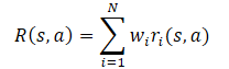
Applying the linearity of the expected value, we find that the Q-function inherits the linear structure from the reward function.
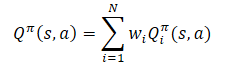
Unless otherwise stated, we assume that Wi=1 for all i. Since the weights of the components are taken out of the Q-function, they can be changed without changing the target forecast of the component. This allows the policy to be evaluated for any combination of weights.
The second point worth paying attention to is that optimizing the decomposed reward function is optimizing the model according to many criteria. It has problems characteristic of multicriteria optimization: conflicting gradients, high curvature and large differences in gradient values. To minimize the negative impact of this factor, the method authors propose to use the Conflict-Averse Gradient Descent (CAGrad) gradient designed for a multi-task reinforcement learning environment. This method aims to mitigate the above problems of multi-objective optimization. The basic idea is to replace the gradient of a multi-task objective function with a weighted sum of the gradients for each individual task. To do this, the following optimization problem is solved:
![]()
where d is an update vector,
g₀ — average gradient,
с — convergence rate coefficient in the range [0, 1).
Solving this optimization problem allows us to take into account the influence of each component on the optimization and focus on improving the worst estimate at each step.
2. Implementation using MQL5
2.1 Creating a new model class
We implement our version of the reward function decomposition based on the SAC+DICE algorithm. Due to the peculiarities of the algorithm implementation, we will not inherit from the CNet_SAC_DICE class created in the previous article. But we will still use the previously made developments. We will create the CNet_SAC_D_DICE class similar to CNet_SAC_DICE. The structure of the new class is provided below.
class CNet_SAC_D_DICE  : protected CNet
  {
protected:
   CNet              cActorExploer;
   CNet              cCritic1;
   CNet              cCritic2;
   CNet              cTargetCritic1;
   CNet              cTargetCritic2;
   CNet              cZeta;
   CNet              cNu;
   CNet              cTargetNu;
   vector<float>     fLambda;
   vector<float>     fLambda_m;
   vector<float>     fLambda_v;
   int               iLatentLayer;
   float             fCAGrad_C;
   int               iCAGrad_Iters;
   int               iUpdateDelay;
   int               iUpdateDelayCount;
   //---
   float             fLoss1;
   float             fLoss2;
   vector<float>     fZeta;
   vector<float>     fQWeights;
   //---
   vector<float>     GetLogProbability(CBufferFloat *Actions);
   vector<float>     CAGrad(vector<float> &grad);

public:
   //---
                     CNet_SAC_D_DICE(void);
                    ~CNet_SAC_D_DICE(void) {}
   //---
   bool              Create(CArrayObj *actor, CArrayObj *critic, CArrayObj *zeta, CArrayObj *nu, int latent_layer = -1);
   //---
   virtual bool      Study(CArrayFloat *State, CArrayFloat *SecondInput, CBufferFloat *Actions, vector<float> &Rewards,
                           CBufferFloat *NextState, CBufferFloat *NextSecondInput, float discount, float tau);
   virtual void      GetLoss(float &loss1, float &loss2)    {  loss1 = fLoss1; loss2 = fLoss2;              }
   virtual bool      TargetsUpdate(float tau);
//---
   virtual void      SetQWeights(vector<float> &weights)    {  fQWeights=weights;                           }
   virtual void      SetCAGradC(float c)                    {  fCAGrad_C=c;                                 }
   virtual void      SetLambda(vector<float> &lambda)       {  fLambda=lambda;
                                                               fLambda_m=vector<float>::Zeros(lambda.Size());
                                                               fLambda_v=fLambda_m;                         }
   virtual void      TargetsUpdateDelay(int delay)          {  iUpdateDelay=delay; iUpdateDelayCount=delay; }
   //---
   virtual bool      Save(string file_name, bool common = true);
   bool              Load(string file_name, bool common = true);
  };
We can see borrowed model objects in the provided class structure. But instead of variables to store the Lagrange coefficient and its averages, we will use vectors whose size is equal to the number of components of the reward function. Here we add the fQWeights vector to store the weighting coefficients of each component. We select the fCAGrad_C variable to record the convergence rate coefficient of the CAGrad method.
Of course, these changes are reflected in the class constructor. At the initial stage, we initialize all vectors of unit length.
CNet_SAC_D_DICE::CNet_SAC_D_DICE(void) :  fLoss1(0),
                                          fLoss2(0),
                                          fCAGrad_C(0.5f),
                                          iCAGrad_Iters(15),
                                          iUpdateDelay(100),
                                          iUpdateDelayCount(100)
  {
   fLambda = vector<float>::Full(1, 1.0e-5f);
   fLambda_m = vector<float>::Zeros(1);
   fLambda_v = vector<float>::Zeros(1);
   fZeta = vector<float>::Zeros(1);
   fQWeights = vector<float>::Ones(1);
  }
The method of initializing a class and creating nested models was taken from the past article without any considerable changes. The changes have been made only to vector sizes.
bool CNet_SAC_D_DICE::Create(CArrayObj *actor, CArrayObj *critic, CArrayObj *zeta, CArrayObj *nu, int latent_layer = -1)
  {
   ResetLastError();
//---
   if(!cActorExploer.Create(actor) || !CNet::Create(actor))
     {
      PrintFormat("Error of create Actor: %d", GetLastError());
      return false;
     }
//---
   if(!opencl)
     {
      Print("Don't opened OpenCL context");
      return false;
     }
//---
   if(!cCritic1.Create(critic) || !cCritic2.Create(critic))
     {
      PrintFormat("Error of create Critic: %d", GetLastError());
      return false;
     }
//---
   if(!cZeta.Create(zeta) || !cNu.Create(nu))
     {
      PrintFormat("Error of create function nets: %d", GetLastError());
      return false;
     }
//---
   if(!cTargetCritic1.Create(critic) || !cTargetCritic2.Create(critic) ||
      !cTargetNu.Create(nu))
     {
      PrintFormat("Error of create target models: %d", GetLastError());
      return false;
     }
//---
   cActorExploer.SetOpenCL(opencl);
   cCritic1.SetOpenCL(opencl);
   cCritic2.SetOpenCL(opencl);
   cZeta.SetOpenCL(opencl);
   cNu.SetOpenCL(opencl);
   cTargetCritic1.SetOpenCL(opencl);
   cTargetCritic2.SetOpenCL(opencl);
   cTargetNu.SetOpenCL(opencl);
//---
   if(!cTargetCritic1.WeightsUpdate(GetPointer(cCritic1), 1.0) ||
      !cTargetCritic2.WeightsUpdate(GetPointer(cCritic2), 1.0) ||
      !cTargetNu.WeightsUpdate(GetPointer(cNu), 1.0))
     {
      PrintFormat("Error of update target models: %d", GetLastError());
      return false;
     }
//---
   cZeta.getResults(fZeta);
   ulong size = fZeta.Size();
   fLambda = vector<float>::Full(size,1.0e-5f);
   fLambda_m = vector<float>::Zeros(size);
   fLambda_v = vector<float>::Zeros(size);
   fQWeights = vector<float>::Ones(size);
   iLatentLayer = latent_layer;
//---
   return true;
  }
Note that here we are initializing the fQWeights bector of weights using single values. If your reward function provides other coefficients, then you need to use the SetQWeights method. However, it should be called after the class has been initialized using the Create method, otherwise your coefficients will be overwritten with single values.
We moved the Conflict-Averse Gradient Descent algorithm into a separate CAGrad method. In the parameters, this method receives a vector of gradients and returns the adjusted vector.
First, we will have to conduct some preparatory work in the method body:
- determine the average value of the gradient;
- scale gradients to improve computational stability;
- prepare local variables and vectors.
vector<float> CNet_SAC_D_DICE::CAGrad(vector<float> &grad)
  {
   matrix<float> GG = grad.Outer(grad);
   GG.ReplaceNan(0);
   if(MathAbs(GG).Sum() == 0)
      return grad;
   float scale = MathSqrt(GG.Diag() + 1.0e-4f).Mean();
   GG = GG / MathPow(scale,2);
   vector<float> Gg = GG.Mean(1);
   float gg = Gg.Mean();
   vector<float> w = vector<float>::Zeros(grad.Size());
   float c = MathSqrt(gg + 1.0e-4f) * fCAGrad_C;
   vector<float> w_best = w;
   float obj_best = FLT_MAX;
   vector<float> moment = vector<float>::Zeros(w.Size());
After completing the preparatory work, we arrange a cycle for solving the optimization problem. In the loop body, we iteratively solve the problem of finding the optimal update vector using the gradient descent method.
   for(int i = 0; i < iCAGrad_Iters; i++)
     {
      vector<float> ww;
      w.Activation(ww,AF_SOFTMAX);
      float obj = ww.Dot(Gg) + c * MathSqrt(ww.MatMul(GG).Dot(ww) + 1.0e-4f);
      if(MathAbs(obj) < obj_best)
        {
         obj_best = MathAbs(obj);
         w_best = w;
        }
      if(i < (iCAGrad_Iters - 1))
        {
         float loss = -obj;
         vector<float> derev = Gg + GG.MatMul(ww) * c / (MathSqrt(ww.MatMul(GG).Dot(ww) + 1.0e-4f) * 2) +
                                    ww.MatMul(GG) * c / (MathSqrt(ww.MatMul(GG).Dot(ww) + 1.0e-4f) * 2);
         vector<float> delta = derev * loss;
         ulong size = delta.Size();
         matrix<float> ident = matrix<float>::Identity(size, size);
         vector<float> ones = vector<float>::Ones(size);
         matrix<float> sm_der = ones.Outer(ww);
         sm_der = sm_der.Transpose() * (ident - sm_der);
         delta = sm_der.MatMul(delta);
         if(delta.Ptp() != 0)
            delta = delta / delta.Ptp();
         moment = delta * 0.8f + moment * 0.5f;
         w += moment;
         if(w.Ptp() != 0)
            w = w / w.Ptp();
        }
     }
After completing the loop iterations, we adjust the error gradients using the optimal weights. The result is returned to the calling program.
   w_best.Activation(w,AF_SOFTMAX);
   float gw_norm = MathSqrt(w.MatMul(GG).Dot(w) + 1.0e-4f);
   float lmbda = c / (gw_norm + 1.0e-4f);
   vector<float> result = ((w * lmbda + 1.0f / (float)grad.Size()) * grad) / (1 + MathPow(fCAGrad_C,2));
//---
   return result;
  }
Just like in the CNet_SAC_DICE class, the entire training is arranged in the CNet_SAC_D_DICE::Study method. But despite the unity of approaches and external similarity, there are many differences in the method algorithm and structure. We made the first changes to the method parameters. Here we have replaced the 'reward' variable with the Rewards vector of decomposed rewards .
Besides, we excluded the ActionsLogProbab action probability logarithm vector. As you know, the Soft Actor-Critic algorithm is used to let the entropy component be included in the reward function to encourage the Agent to repeat low-probability actions. The decomposition of the reward function allocates a separate element for each component. Thus, the probability logarithms are already present in the Rewards decomposed reward vector and we do not need to duplicate them in a separate vector.
bool CNet_SAC_D_DICE::Study(CArrayFloat *State,
                            CArrayFloat *SecondInput,
                            CBufferFloat *Actions,
                            vector<float> &Rewards,
                            CBufferFloat *NextState,
                            CBufferFloat *NextSecondInput,
                            float discount,
                            float tau)
  {
//---
   if(!Actions)
      return false;
In the method body, we check the relevance of the pointer to the resulting buffer of completed actions. This concludes the control block of our method.
Moving on to the next stage, it must be said that in the process of training the model, a rather large unreasonable increase in the estimates of subsequent states by the target models was noticed. Such estimates greatly exceeded the actual rewards, which led to mutual adaptation of the trained model and its target copy without taking into account the actual rewards of the environment.
To minimize this effect, it was decided to train the model using the actual cumulative reward at the initial stage. A complete refusal to use target models also has a negative effect. In the experience replay buffer, the cumulative assessment is limited to a training period. It can be very different for similar states and actions depending on the distance to the end of the training set. This difference is smoothed out by the target model. In addition, the target model helps estimate states based on current policy actions. As the number of iterations of updating Agent parameters increases, the current policy will increasingly differ from the policy in the experience playback buffer, which cannot be ignored. But we need a target model with adequate estimates. Thus, we need two modes of the method operation: with and without the use of target models.
While arranging the method algorithm, we are guided by the following considerations:
- If it is necessary to use target models, the user passes pointers to future states in the parameters. The Rewards vector contains a decomposed reward only for the action performed in the current state.
- After refusing the use of target models, a user does not pass the pointers to future states (the parameter variables contain NULL). The Rewards vector contains a cumulative decomposed reward.
Therefore, we next check the pointer to the future state and, if necessary, determine an action in the future state based on the current policy. Besides, we evaluate the state-action pair.
   if(!!NextState)
      if(!CNet::feedForward(NextState, 1, false, NextSecondInput))
         return false;
   if(!cTargetCritic1.feedForward(GetPointer(this), iLatentLayer, GetPointer(this), layers.Total() - 1) ||
      !cTargetCritic2.feedForward(GetPointer(this), iLatentLayer, GetPointer(this), layers.Total() - 1))
      return false;
//---
   if(!cTargetNu.feedForward(GetPointer(this), iLatentLayer, GetPointer(this), layers.Total() - 1))
      return false;
Next, we take a direct pass of the conservative policy in the current state. Replace actions and carry out a direct pass through the DICE block models.
   if(!CNet::feedForward(State, 1, false, SecondInput))
      return false;
   CBufferFloat *output = ((CNeuronBaseOCL*)((CLayer*)layers.At(layers.Total() - 1)).At(0)).getOutput();
   output.AssignArray(Actions);
   output.BufferWrite();
   if(!cNu.feedForward(GetPointer(this), iLatentLayer, GetPointer(this)))
      return false;
   if(!cZeta.feedForward(GetPointer(this), iLatentLayer, GetPointer(this)))
      return false;
Next, determine the values of the loss functions of the Distribution Correction Estimation block models. This step was described in detail in the previous article. I just emphasize that in case of refusal to use the target model, the vector for assessing the future state next_nu is filled with zero values.
   vector<float> nu, next_nu, zeta, ones;
   cNu.getResults(nu);
   cZeta.getResults(zeta);
   if(!!NextState)
      cTargetNu.getResults(next_nu);
   else
      next_nu = vector<float>::Zeros(nu.Size());
   ones = vector<float>::Ones(zeta.Size());
   vector<float> log_prob = GetLogProbability(output);
   int shift = (int)(Rewards.Size() - log_prob.Size());
   if(shift < 0)
      return false;
   float policy_ratio = 0;
   for(ulong i = 0; i < log_prob.Size(); i++)
      policy_ratio += log_prob[i] - Rewards[shift + i] / LogProbMultiplier;
   policy_ratio = MathExp(policy_ratio / log_prob.Size());
   vector<float> bellman_residuals = (next_nu * discount + Rewards) * policy_ratio - nu;
   vector<float> zeta_loss = MathPow(zeta, 2.0f) / 2.0f - zeta * (MathAbs(bellman_residuals) - fLambda) ;
   vector<float> nu_loss = zeta * MathAbs(bellman_residuals) + MathPow(nu, 2.0f) / 2.0f;
   vector<float> lambda_los = fLambda * (ones - zeta);
Next, we update the vector of Lagrange coefficients using the Adam optimization method.
Please note that we correct the vector of error gradients using the CAGrad method discussed above. The use of vector operations allows us to work with vectors as simply as with simple variables.
We will save the adjusted values in the corresponding vector.
   vector<float> grad_lambda = CAGrad((ones - zeta) * (lambda_los * (-1.0f)));
   fLambda_m = fLambda_m * b1 + grad_lambda * (1 - b1);
   fLambda_v = fLambda_v * b2 + MathPow(grad_lambda, 2) * (1.0f - b2);
   fLambda += fLambda_m * lr / MathSqrt(fLambda_v + lr / 100.0f);
The next step is updating the v, ζ model parameters. The algorithm for these operations remains the same. We just replace variables with vectors and use vector operations.
   CBufferFloat temp;
   temp.BufferInit(MathMax(Actions.Total(), SecondInput.Total()), 0);
   temp.BufferCreate(opencl);
//--- update nu
   int last_layer = cNu.layers.Total() - 1;
   CLayer *layer = cNu.layers.At(last_layer);
   if(!layer)
      return false;
   CNeuronBaseOCL *neuron = layer.At(0);
   if(!neuron)
      return false;
   CBufferFloat *buffer = neuron.getGradient();
   if(!buffer)
      return false;
   vector<float> nu_grad = CAGrad(nu_loss * (zeta * bellman_residuals / MathAbs(bellman_residuals) - nu));
   if(!buffer.AssignArray(nu_grad) || !buffer.BufferWrite())
      return false;
   if(!cNu.backPropGradient(output, GetPointer(temp)))
      return false;
We necessarily correct the vectors of error gradients using the Conflict-Averse Gradient Descent algorithm in the CNet_SAC_D_DICE::CAGrad method.
//--- update zeta
   last_layer = cZeta.layers.Total() - 1;
   layer = cZeta.layers.At(last_layer);
   if(!layer)
      return false;
   neuron = layer.At(0);
   if(!neuron)
      return false;
   buffer = neuron.getGradient();
   if(!buffer)
      return false;
   vector<float> zeta_grad = CAGrad(zeta_loss * (zeta - MathAbs(bellman_residuals) + fLambda) * (-1.0f));
   if(!buffer.AssignArray(zeta_grad) || !buffer.BufferWrite())
      return false;
   if(!cZeta.backPropGradient(output, GetPointer(temp)))
      return false;
At this stage, we finish working with the objects of the Distribution Correction Estimation block and move on to training our Critic models. First, we carry out their forward pass. We have already carried out the forward passage of the Actor earlier.
//--- feed forward critics
   if(!cCritic1.feedForward(GetPointer(this), iLatentLayer, output) ||
      !cCritic2.feedForward(GetPointer(this), iLatentLayer, output))
      return false;
The next step is to determine the vector of reference values for updating the Critics parameters. There are two nuances here. Both of them concern target models. First, we test the need for their use to assess subsequent state and action. To do this, we check a pointer to the subsequent state of the system.
If we do use target models to evaluate the subsequent state-action pair, then we need to select the target Critic with the minimum cumulative score. The cumulative estimate is easily obtained by multiplying the vector of weighting coefficients of the reward function components by the vector of decomposed predictive reward obtained from a forward pass of the target models. Next, all we have to do is select the minimum estimate and save the vector of predicted values of the selected model.
If you refuse to evaluate subsequent states, the vector of predicted values is filled with zero values.
   vector<float> result;
   if(fZeta.CompareByDigits(vector<float>::Zeros(fZeta.Size()),8) == 0)
      fZeta = MathAbs(zeta);
   else
      fZeta = fZeta * 0.9f + MathAbs(zeta) * 0.1f;
   zeta = MathPow(MathAbs(zeta), 1.0f / 3.0f) / (MathPow(fZeta, 1.0f / 3.0f) * 10.0f);
   vector<float> target = vector<float>::Zeros(Rewards.Size());
   if(!!NextState)
     {
      cTargetCritic1.getResults(target);
      cTargetCritic2.getResults(result);
      if(fQWeights.Dot(result) < fQWeights.Dot(target))
         target = result;
     }
Adjust the forecast estimates by the discount factor and sum them up with the reward of the current state.
   target = (target * discount + Rewards);
   ulong total = log_prob.Size();
   for(ulong i = 0; i < total; i++)
      target[shift + i] = log_prob[i] * LogProbMultiplier;
In the resulting vector, we will adjust the action probability logarithm in the current policy. The logarithms of action probabilities stored in the experience replay buffer are already contained in the reward vector. We replace their values with logarithms of current policy in order to train the critic to make assessments taking the current policy into account.
After determining the target values, we calculate the prediction error of the first Critic and the error gradient for each component of the Q-function. The resulting gradients are adjusted using the Conflict-Averse Gradient Descent algorithm.
//--- update critic1
   cCritic1.getResults(result);
   vector<float> loss = zeta * MathPow(result - target, 2.0f);
   if(fLoss1 == 0)
      fLoss1 = MathSqrt(fQWeights.Dot(loss) / fQWeights.Sum());
   else
      fLoss1 = MathSqrt(0.999f * MathPow(fLoss1, 2.0f) + 0.001f * fQWeights.Dot(loss) / fQWeights.Sum());
   vector<float> grad = CAGrad(loss * zeta * (target - result) * 2.0f);
We transfer the corrected error gradients to the corresponding Critic1 buffer and perform a reverse model pass.
   last_layer = cCritic1.layers.Total() - 1;
   layer = cCritic1.layers.At(last_layer);
   if(!layer)
      return false;
   neuron = layer.At(0);
   if(!neuron)
      return false;
   buffer = neuron.getGradient();
   if(!buffer)
      return false;
   if(!buffer.AssignArray(grad) || !buffer.BufferWrite())
      return false;
   if(!cCritic1.backPropGradient(output, GetPointer(temp)) ||
      !backPropGradient(SecondInput, GetPointer(temp), iLatentLayer))
      return false;
Here we also carry out a partial reverse pass of the Actor to adjust the block of prep-processing the source data.
Repeat the operations for the second Critic.
//--- update critic2
   cCritic2.getResults(result);
   loss = zeta * MathPow(result - target, 2.0f);
   if(fLoss2 == 0)
      fLoss2 = MathSqrt(fQWeights.Dot(loss) / fQWeights.Sum());
   else
      fLoss2 = MathSqrt(0.999f * MathPow(fLoss2, 2.0f) + 0.001f * fQWeights.Dot(loss) / fQWeights.Sum());
   grad = CAGrad(loss * zeta * (target - result) * 2.0f);
   last_layer = cCritic2.layers.Total() - 1;
   layer = cCritic2.layers.At(last_layer);
   if(!layer)
      return false;
   neuron = layer.At(0);
   if(!neuron)
      return false;
   buffer = neuron.getGradient();
   if(!buffer)
      return false;
   if(!buffer.AssignArray(grad) || !buffer.BufferWrite())
      return false;
   if(!cCritic2.backPropGradient(output, GetPointer(temp)) ||
      !backPropGradient(SecondInput, GetPointer(temp), iLatentLayer))
      return false;
In the next block of our method, we will update the policies. Let me remind you that the SAC+DICE algorithm provides for training two Actor policies: conservative and optimistic. First, we will update the conservative policy. We have already carried out the forward pass for this model.
To train the Actors, we will use the minimum average error Critic. Let's define such a model and store a pointer to it in a local variable.
   vector<float> mean;
   CNet *critic = NULL;
   if(fLoss1 <= fLoss2)
     {
      cCritic1.getResults(result);
      cCritic2.getResults(mean);
      critic = GetPointer(cCritic1);
     }
   else
     {
      cCritic1.getResults(mean);
      cCritic2.getResults(result);
      critic = GetPointer(cCritic2);
     }
Here we will upload the predicted ratings of each of the Critics. Then we will determine the reference values for the reverse pass of the models using the equation.
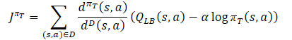
At the same time, we make sure to correct the vector of error gradients using the Conflict-Averse Gradient Descent method.
   vector<float> var = MathAbs(mean - result) / 2.0f;
   mean += result;
   mean /= 2.0f;
   target = mean;
   for(ulong i = 0; i < log_prob.Size(); i++)
      target[shift + i] = discount * log_prob[i] * LogProbMultiplier;
   target = CAGrad(zeta * (target - var * 2.5f) - result) + result;
Next, we just need to transfer the received data to the buffer and perform a reverse pass of the Critic and the Actor. To prevent mutual adjustment of models, turn off the Critic training mode before starting the operations. In this case, we only use it to pass the error gradient to the Actor.
   CBufferFloat bTarget;
   bTarget.AssignArray(target);
   critic.TrainMode(false);
   if(!critic.backProp(GetPointer(bTarget), GetPointer(this)) ||
      !backPropGradient(SecondInput, GetPointer(temp)))
     {
      critic.TrainMode(true);
      return false;
     }
We have not yet used the model of an optimistic Actor, in contrast to a conservative one. Therefore, before starting the update of its parameters, we have to carry out a direct pass with the current state of the environment.
//--- update exploration policy
   if(!cActorExploer.feedForward(State, 1, false, SecondInput))
     {
      critic.TrainMode(true);
      return false;
     }
   output = ((CNeuronBaseOCL*)((CLayer*)cActorExploer.layers.At(layers.Total() - 1)).At(0)).getOutput();
   output.AssignArray(Actions);
   output.BufferWrite();
As in the case of a conservative Actor, we replace the vector of actions and obtain logarithms of probabilities, while taking into account the optimistic policy.
cActorExploer.GetLogProbs(log_prob);
Determine the vector of reference values for the reverse pass of the models according to the optimistic policy equation.
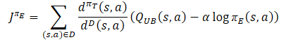
The vector of error gradients is corrected using the Conflict-Averse Gradient Descent method.
   target = mean;
   for(ulong i = 0; i < log_prob.Size(); i++)
      target[shift + i] = discount * log_prob[i] * LogProbMultiplier;
   target = CAGrad(zeta * (target + var * 2.0f) - result) + result;
Then we perform a reverse pass through the models and return the Critic to the model training mode.
   bTarget.AssignArray(target);
   if(!critic.backProp(GetPointer(bTarget), GetPointer(cActorExploer)) ||
      !cActorExploer.backPropGradient(SecondInput, GetPointer(temp)))
     {
      critic.TrainMode(true);
      return false;
     }
   critic.TrainMode(true);
Next we need to update the target models. Here I made further additions to prevent distortion of estimates of future states and adaptation of Critics’ models to the values of their target copies.
The parameters of the target models are updated at each iteration only if they are no longer used to estimate the subsequent state. If the target models are used in training, then their update is carried out with a delay.
Therefore, we first check the need to update models and only then carry out operations.
   if(!!NextState)
     {
      if(iUpdateDelayCount > 0)
        {
         iUpdateDelayCount--;
         return true;
        }
      iUpdateDelayCount = iUpdateDelay;
     }
   if(!cTargetCritic1.WeightsUpdate(GetPointer(cCritic1), tau) ||
      !cTargetCritic2.WeightsUpdate(GetPointer(cCritic2), tau) ||
      !cTargetNu.WeightsUpdate(GetPointer(cNu), tau))
     {
      PrintFormat("Error of update target models: %d", GetLastError());
      return false;
     }
//---
   return true;
  }
After successful completion of all iterations of the method, we terminate its work with the 'true' result.
The decomposition of rewards and the use of vectors led to changes in other methods, including the ones of working with files. But we will not dwell on them now. You can find them, as well as the full code of all methods of the new class, in the attached file "MQL5\Experts\SAC-D&DICE\Net_SAC_D_DICE.mqh".
2.2 Adjusting the data storage structures
NOw let's focus our attention on the "MQL5\Experts\SAC-D&DICE\Trajectory.mqh" file. We used to change the architecture of the models here. Now we have left it practically unchanged. We only need to change the number of neurons at the Critic output. They should be sufficient to decompose the reward function. But before specifying their number, let's define the structure of the decomposed reward.
We will indicate the relative change in balance in the first element with index "0". As you know, our main goal is to maximize profits in the market.
The parameter with index "1" will contain the relative value of the Equity change. A negative value indicates an unwanted drawdown. A positive one shows a floating profit.
One more element is allocated for penalties for the lack of open positions.
Next, add the logarithms of action probabilities. As you know, the length of the probability logarithm vector is equal to the action vector.
//+------------------------------------------------------------------+
//| Rewards structure                                                |
//|   0     -  Delta Balance                                         |
//|   1     -  Delta Equity ( "-" Drawdown / "+" Profit)             |
//|   2     -  Penalty for no open positions                         |
//|   3...  -  LogProbs vector                                       |
//+------------------------------------------------------------------+
Thus, the size of the neural layer of the Critic results is 3 elements greater than the number of actions.
#define                    NActions        6            //Number of possible Actions
#define                    NRewards        3+NActions   //Number of rewards
bool CreateDescriptions(CArrayObj *actor, CArrayObj *critic)
  {
//---
   CLayerDescription *descr;
//---
   if(!actor)
     {
      actor = new CArrayObj();
      if(!actor)
         return false;
     }
   if(!critic)
     {
      critic = new CArrayObj();
      if(!critic)
         return false;
     }
//--- Actor
........
........
//--- Critic
   critic.Clear();
//--- Input layer
........
........
//--- layer 4
   if(!(descr = new CLayerDescription()))
      return false;
   descr.type = defNeuronBaseOCL;
   descr.count = NRewards;
   descr.optimization = ADAM;
   descr.activation = None;
   if(!critic.Add(descr))
     {
      delete descr;
      return false;
     }
//---
   return true;
  }
The reward decomposition also changed the structure of data storage in the experience replay buffer. Now one variable is not enough for us to set the reward. We need a data array. At the same time, we have introduced the entropy component into the reward array and we do not need a separate array to reset these values. Therefore, in the state description structure, we replace the 'log_prob' array with 'rewards' and adjust the methods for copying the structure and handling the files.
struct SState
  {
   float             state[HistoryBars * BarDescr];
   float             account[AccountDescr - 4];
   float             action[NActions];
   float             rewards[NRewards];
   //---
                     SState(void);
   //---
   bool              Save(int file_handle);
   bool              Load(int file_handle);
   //--- overloading
   void              operator=(const SState &obj)
     {
      ArrayCopy(state, obj.state);
      ArrayCopy(account, obj.account);
      ArrayCopy(action, obj.action);
      ArrayCopy(rewards, obj.rewards);
     }
  };
In the STrajectory trajectory structure, delete the Rewards array, since we will now describe the reward in the SState state structure. Also, let's make targeted changes to the structure methods.
struct STrajectory
  {
   SState            States[Buffer_Size];
   int               Total;
   float             DiscountFactor;
   bool              CumCounted;
   //---
                     STrajectory(void);
   //---
   bool              Add(SState &state);
   void              CumRevards(void);
   //---
   bool              Save(int file_handle);
   bool              Load(int file_handle);
  };
The full code of the mentioned structures and their methods is available in the attachment.
2.3 Creating model training EAs
It is time to work on model training EAs. During the training, we use three EAs as before:
- Research — collecting example database
- Study — model training
- Test — checking obtained results.
In the Research and Test EAs, the changes affected only the preparation of the environment state description structure and the reward received at the end of the OnTick method. While we summed up rewards and fines previously, now we add each component to its own array element. In this case, it is important to comply with the above data structure. Each element of the array must be filled in. If the component value is missing, then write "0" to the corresponding array element. This approach will give us confidence in the validity of the data used.
void OnTick()
  {
//---
........
........
//---
   sState.rewards[0] = bAccount[0];
   sState.rewards[1] = 1.0f-bAccount[1];
   vector<float> log_prob;
   Actor.GetLogProbs(log_prob);
   if((buy_value + sell_value) == 0)
      sState.rewards[2] -= (float)(atr / PrevBalance);
   else
      sState.rewards[2] = 0;
   for(ulong i = 0; i < NActions; i++)
     {
      sState.action[i] = ActorResult[i];
      sState.rewards[i + 3] = log_prob[i] * LogProbMultiplier;
     }
   if(!Base.Add(sState))
      ExpertRemove();
  }
The full codes of EAs can be found in the attachment.
As usual, the model training is carried out in the Study EA. As mentioned above, we divide the process of training models into two stages:
- Training with actual cumulative reward (no target models),
- Training using target models.
The duration of the first stage is determined by a constant.
#define StartTargetIteration 20000
It is worth noting that training without using target models is carried out only when you first launch the Study EA, when there are no pre-trained models.
If, at startup, the training EA managed to load pre-trained models, then the target models are used from the first training iteration.
This control is implemented in the EA's OnInit method.
int OnInit()
  {
//---
   ResetLastError();
   if(!LoadTotalBase())
     {
      PrintFormat("Error of load study data: %d", GetLastError());
      return INIT_FAILED;
     }
//--- load models
   if(!Net.Load(FileName, true))
     {
      CArrayObj *actor = new CArrayObj();
      CArrayObj *critic = new CArrayObj();
      if(!CreateDescriptions(actor, critic))
        {
         delete actor;
         delete critic;
         return INIT_FAILED;
        }
      if(!Net.Create(actor, critic, critic, critic, LatentLayer))
        {
         delete actor;
         delete critic;
         return INIT_FAILED;
        }
      delete actor;
      delete critic;
      StartTargetIter = StartTargetIteration;
     }
   else
      StartTargetIter = 0;
//---
   if(!EventChartCustom(ChartID(), 1, 0, 0, "Init"))
     {
      PrintFormat("Error of create study event: %d", GetLastError());
      return INIT_FAILED;
     }
//---
   return(INIT_SUCCEEDED);
  }
As you can see, the StartTargetIter variable receives the StartTargetIteration constant value when creating new models. If pre-trained models are loaded, then we store "0" in the delay variable.
The training iterations are arranged in the Train method. At the beginning of the method, we, as usual, determine the number of saved trajectories in the experience replay buffer and arrange a training loop with the number of iterations specified in the EA external parameter.
void Train(void)
  {
   int total_tr = ArraySize(Buffer);
   uint ticks = GetTickCount();
//---
   for(int iter = 0; (iter < Iterations && !IsStopped()); iter ++)
     {
      int tr = (int)((MathRand() / 32767.0) * (total_tr - 1));
      int i = (int)((MathRand() * MathRand() / MathPow(32767, 2)) * (Buffer[tr].Total - 2));
      if(i < 0)
        {
         iter--;
         continue;
        }
In the body of the loop, we randomly sample the state in one of the saved trajectories. After that, we pass information about the selected state to the data buffers and the vector.
      //---
      bState.AssignArray(Buffer[tr].States[i].state);
      float PrevBalance = Buffer[tr].States[MathMax(i - 1, 0)].account[0];
      float PrevEquity = Buffer[tr].States[MathMax(i - 1, 0)].account[1];
      bAccount.Clear();
      bAccount.Add((Buffer[tr].States[i].account[0] - PrevBalance) / PrevBalance);
      bAccount.Add(Buffer[tr].States[i].account[1] / PrevBalance);
      bAccount.Add((Buffer[tr].States[i].account[1] - PrevEquity) / PrevEquity);
      bAccount.Add(Buffer[tr].States[i].account[2]);
      bAccount.Add(Buffer[tr].States[i].account[3]);
      bAccount.Add(Buffer[tr].States[i].account[4] / PrevBalance);
      bAccount.Add(Buffer[tr].States[i].account[5] / PrevBalance);
      bAccount.Add(Buffer[tr].States[i].account[6] / PrevBalance);
      double x = (double)Buffer[tr].States[i].account[7] / (double)(D'2024.01.01' - D'2023.01.01');
      bAccount.Add((float)MathSin(x != 0 ? 2.0 * M_PI * x : 0));
      x = (double)Buffer[tr].States[i].account[7] / (double)PeriodSeconds(PERIOD_MN1);
      bAccount.Add((float)MathCos(x != 0 ? 2.0 * M_PI * x : 0));
      x = (double)Buffer[tr].States[i].account[7] / (double)PeriodSeconds(PERIOD_W1);
      bAccount.Add((float)MathSin(x != 0 ? 2.0 * M_PI * x : 0));
      x = (double)Buffer[tr].States[i].account[7] / (double)PeriodSeconds(PERIOD_D1);
      bAccount.Add((float)MathSin(x != 0 ? 2.0 * M_PI * x : 0));
      //---
      bActions.AssignArray(Buffer[tr].States[i].action);
      vector<float> rewards;
      rewards.Assign(Buffer[tr].States[i].rewards);
Please note that at the current stage we only prepare information about the selected state. In order not to perform unnecessary work, we will generate information about the subsequent state only if necessary.
We test the need to use target models to estimate the subsequent state by comparing the current training iteration and the value of the StartTargetIter variable. If the number of iterations has not reached the threshold value, then we carry out training on cumulative values. But there is a nuance here. When saving data to the experience playback buffer, we calculated the cumulative total of the values of all reward components. However, we need the entropy component without a cumulative total. Therefore, we arrange a loop and remove the accumulated values only from the entropy component of the reward function.
      //---
      if(iter < StartTargetIter)
        {
         ulong start = rewards.Size() - bActions.Total();
         for(ulong r = start; r < rewards.Size(); r++)
            rewards[r] -= Buffer[tr].States[i + 1].rewards[r] * DiscFactor;
         if(!Net.Study(GetPointer(bState), GetPointer(bAccount), GetPointer(bActions), rewards,
                       NULL, NULL, DiscFactor, Tau))
           {
            PrintFormat("%s -> %d", __FUNCTION__, __LINE__);
            break;
           }
        }
Then we call the training method of our new class. Here we specify "NULL" in the subsequent state parameters.
After reaching the threshold of using the objective functions, we will first prepare information about the subsequent state of the system.
      else
        {
         //--- Target
         bNextState.AssignArray(Buffer[tr].States[i + 1].state);
         PrevBalance = Buffer[tr].States[i].account[0];
         PrevEquity = Buffer[tr].States[i].account[1];
         if(PrevBalance == 0)
           {
            iter--;
            continue;
           }
         bNextAccount.Clear();
         bNextAccount.Add((Buffer[tr].States[i + 1].account[0] - PrevBalance) / PrevBalance);
         bNextAccount.Add(Buffer[tr].States[i + 1].account[1] / PrevBalance);
         bNextAccount.Add((Buffer[tr].States[i + 1].account[1] - PrevEquity) / PrevEquity);
         bNextAccount.Add(Buffer[tr].States[i + 1].account[2]);
         bNextAccount.Add(Buffer[tr].States[i + 1].account[3]);
         bNextAccount.Add(Buffer[tr].States[i + 1].account[4] / PrevBalance);
         bNextAccount.Add(Buffer[tr].States[i + 1].account[5] / PrevBalance);
         bNextAccount.Add(Buffer[tr].States[i + 1].account[6] / PrevBalance);
         x = (double)Buffer[tr].States[i + 1].account[7] / (double)(D'2024.01.01' - D'2023.01.01');
         bNextAccount.Add((float)MathSin(x != 0 ? 2.0 * M_PI * x : 0));
         x = (double)Buffer[tr].States[i + 1].account[7] / (double)PeriodSeconds(PERIOD_MN1);
         bNextAccount.Add((float)MathCos(x != 0 ? 2.0 * M_PI * x : 0));
         x = (double)Buffer[tr].States[i + 1].account[7] / (double)PeriodSeconds(PERIOD_W1);
         bNextAccount.Add((float)MathSin(x != 0 ? 2.0 * M_PI * x : 0));
         x = (double)Buffer[tr].States[i + 1].account[7] / (double)PeriodSeconds(PERIOD_D1);
         bNextAccount.Add((float)MathSin(x != 0 ? 2.0 * M_PI * x : 0));
Then we remove the cumulative values for all components of the reward function, leaving only the rewards of the current state.
         for(ulong r = 0; r < rewards.Size(); r++)
            rewards[r] -= Buffer[tr].States[i + 1].rewards[r] * DiscFactor;
         if(!Net.Study(GetPointer(bState), GetPointer(bAccount), GetPointer(bActions), rewards,
                       GetPointer(bNextState), GetPointer(bNextAccount), DiscFactor, Tau))
           {
            PrintFormat("%s -> %d", __FUNCTION__, __LINE__);
            break;
           }
        }
Call the training method for the class model. This time we specify objects with subsequent state data.
At the end of a loop iteration, we print a message to inform the user and move on to the next iteration.
      //---
      if(GetTickCount() - ticks > 500)
        {
         float loss1, loss2;
         Net.GetLoss(loss1, loss2);
         string str = StringFormat("%-15s %5.2f%% -> Error %15.8f\n", "Critic1",
                                                                    iter * 100.0 / (double)(Iterations), loss1);
         str += StringFormat("%-15s %5.2f%% -> Error %15.8f\n", "Critic2",
                                                                    iter * 100.0 / (double)(Iterations), loss2);
         Comment(str);
         ticks = GetTickCount();
        }
     }
After successfully completing all loop iterations, clear the comments field on the chart. Force update the target models. Display the training result to the MetaTrader 5 journal and initiate the EA shutdown.
   Comment("");
//---
   float loss1, loss2;
   Net.GetLoss(loss1, loss2);
   Net.TargetsUpdate(Tau);
   PrintFormat("%s -> %d -> %-15s %10.7f", __FUNCTION__, __LINE__, "Critic1", loss1);
   PrintFormat("%s -> %d -> %-15s %10.7f", __FUNCTION__, __LINE__, "Critic2", loss2);
   ExpertRemove();
//---
  }
This concludes our work with the model training EAs. The full code of all programs used in the article is available in the attachment.
3. Test
We have proposed an option for the implementation of the reward function decomposition approach based on the SAC+DICE algorithm, and now we can evaluate the results of the work done in practice. As before, the models were trained on EURUSD H1 on the first 5 months of 2023. All indicator parameters are used by default. The initial balance is USD 10,000.
The model training process is iterative, alternating with the stages of collecting examples into an experience accumulation buffer and updating the model parameters.
At the first stage, we create a primary database of examples using Actor models filled with random parameters. As a result, we get a series of random passes that generate off-policy "State → Action → New state → Reward" data sets.
Unlike all previously considered algorithms, in this case we collect decomposed data on the environment rewards for the Agent’s actions.
After collecting examples, we carry out initial training of our model. To achieve this, we launch the "..\SAC-D&DICE\Study.mq5" EA.
During the primary training without using target models, we observe a steady trend towards a decrease in the errors of both Critics. However, when using target models to estimate the subsequent state, chaotic (infrequent) spikes in prediction error are observed followed by a smooth return to the previous error level.
At the second stage, we re-launch the training data collection EA in the optimization mode of the strategy tester with a complete search of parameters. This time, we use the optimistic Actor, trained at the first stage, for all passes. The scatter of the results of individual passes is lower than the initial data collection and is due to the stochasticity of the Actor’s policy.
Collecting examples and training the model are repeated several times until the desired result is obtained or a local minimum is reached when the next iteration of collecting examples and training the model does not produce any progress.
While training the model, we obtained an Actor policy capable of generating a small profit during the training period.


Despite the profit received, the learned policy is far from what we want. On the balance graph, we see a wave-like movement with a fairly large amplitude. Only 32% of 28 trades were closed with a profit. The total profit was achieved due to the excess of the size of a profitable trade over a losing one. The average profit on a trade exceeds the average loss 2 times. The maximum profit per trade is almost 3.5 times the maximum loss. As a result, the profit factor is slightly higher than 1.
The EA also showed profit on the new data. In one month after the training period, the model was able to receive almost 20% of the profit, which is higher than the result on the training set. However, the statistics of the results are comparable to the training set data. During the test, only 4 trades were made and only one of them was closed with a profit. But the profit on this trade is 12.8 times higher than the worst one of the losing trades.


Comparing the results on the training sample and on the subsequent period, we can assume that we are observing the beginning of a wave of profitability on the new data, which may be followed by a decline in the foreseeable future.
Overall, the model is capable of generating profits, but additional optimization is required.
Conclusion
In this article, we introduced the reward function decomposition approach, which allows us to train Agents more efficiently. Reward decomposition allows users to analyze the influence of various components on the decisions made by the Agent.
We have implemented the algorithm using MQL5 and integrated the decomposition of the reward function into the SAC+DICE method.
While testing the implemented algorithm, we managed to obtain a model capable of generating profit both on the training set and outside it. This indicates the generalizing ability of the algorithm.
However, the results obtained are far from what we want. At the same time, decomposition of the reward function makes it possible to analyze the influence of individual components of the reward function on the training outcome. I encourage you to experiment with including and excluding individual components to evaluate their impact on the training outcome.
Links
- Conflict-Averse Gradient Descent for Multi-task Learning
- Value Function Decomposition for Iterative Design of Reinforcement Learning Agents
- Neural networks made easy (Part 52): Research with optimism and distribution correction
Programs used in the article
| # | Name | Type | Description |
|---|---|---|---|
| 1 | Research.mq5 | Expert Advisor | Example collection EA |
| 2 | Study.mq5 | Expert Advisor | Agent training EA |
| 3 | Test.mq5 | Expert Advisor | Model testing EA |
| 4 | Trajectory.mqh | Class library | System state description structure |
| 5 | Net_SAC_D_DICE.mqh | Class library | Model class |
| 6 | NeuroNet.mqh | Class library | A library of classes for creating a neural network |
| 7 | NeuroNet.cl | Code Base | OpenCL program code library |
Translated from Russian by MetaQuotes Ltd.
Original article: https://www.mql5.com/ru/articles/13098
Warning: All rights to these materials are reserved by MetaQuotes Ltd. Copying or reprinting of these materials in whole or in part is prohibited.
This article was written by a user of the site and reflects their personal views. MetaQuotes Ltd is not responsible for the accuracy of the information presented, nor for any consequences resulting from the use of the solutions, strategies or recommendations described.

- Free trading apps
- Over 8,000 signals for copying
- Economic news for exploring financial markets
You agree to website policy and terms of use
Thank you Dmitry, I clicked on your seller profile hoping to find some nn EAs I could test.
I have taken a udemy MQL5 course on nn, now trying to go deeper. I am Starting with your series of articles.