Python, ONNX and MetaTrader 5: Creating a RandomForest model with RobustScaler and PolynomialFeatures data preprocessing

What base are we going to use? What is Random Forest?

The history of the development of the Random Forest method goes back a long way and is associated with the work of prominent scientists in the field of machine learning and statistics. To better understand the principles and application of this method, let's imagine it as a huge group of people (decision trees) who work together.

The random forest method has its roots in decision trees. Decision trees serve as a graphical representation of a decision-making algorithm, where each node represents a test on one of the attributes, each branch is the result of that test, and the leaves are the predicted output. Decision trees were developed in the mid-20th century and have become popular classification and regression tools.

The next important step was the concept of bagging (Bootstrap Aggregating), proposed by Leo Breiman in 1996. Bagging implies splitting a training dataset into multiple bootstrap samples (subsamples) and training separate models on each of them. The models' results are then averaged or combined to produce more robust and accurate predictions. This method has enabled the reduction in the model variance and the improvement of their generalization ability.

The Random Forest method was proposed by Leo Breiman and Adele Cutler in the early 2000s. It is based on the idea of combining multiple decision trees using bagging and additional randomness. Each tree is built from a random subsample of the training dataset, and a random set of features is selected when building each node in the tree. This makes each tree unique and reduces the correlation between trees, resulting in improved generalization ability.

Random Forest has quickly become one of the most popular methods in machine learning due to its high performance and ability to handle both classification and regression problems. In classification problems, it is used to make decisions about which class an object belongs to, and in regression it is used to predict numerical values.

Today, Random Forest is widely used in various fields including finance, medicine, data analytics and many others. It is appreciated for its robustness and ability to handle complex machine learning problems.

Random Forest is a powerful tool in the machine learning toolkit. To better understand how it works, let's visualize it as a huge group of people coming together and making collective decisions. However, instead of real people, each member in this group is an independent classifier or predictor of the current situation. Within this group, a person is a decision tree capable of making decisions based on certain attributes. When the random forest makes a decision, it uses democracy and voting: each tree expresses its opinion, and the decision is made based on multiple votes.

Random Forest is widely used in a variety of fields, and its flexibility makes it suitable for both classification and regression problems. In a classification task, the model decides which of the predefined classes the current state belongs to. For example, in the financial market, this could mean a decision to buy (class 1) or sell (class 0) an asset based on a variety of indicators.

However, in this article, we will focus on regression problems. Regression in machine learning is an attempt to predict the future numerical values of a time series based on its past values. Instead of classification, where we assign objects to certain classes, in regression we aim to predict specific numbers. This could be, for example, forecasting stock prices, predicting temperature or any other numerical variable.

Creating a Basic RF Model

To create a basic Random Forest model, we will use the sklearn (Scikit-learn) library in Python. Below is a simple code template for training a Random Forest regression model. Before running this code, you should install the libraries needed to run sklearn using the Python Package Installer tool.

pip install onnx
pip install skl2onnx
pip install MetaTrader5

Next, it is necessary to import libraries and set parameters. We import the necessary libraries, including 'pandas' for working with data, 'gdown' for loading data from Google Drive, as well as libraries for data processing and creating a Random Forest model. We also set the number of time steps (n_steps) in the data sequence, which is determined depending on the specific requirements:

import pandas as pd
import gdown
import numpy as np
import joblib
import random
import onnx
import os
import shutil
from sklearn.ensemble import RandomForestRegressor
from sklearn.metrics import mean_squared_error, r2_score
from sklearn.utils import shuffle
from skl2onnx import convert_sklearn
from skl2onnx.common.data_types import FloatTensorType
from sklearn.pipeline import Pipeline
from sklearn.preprocessing import RobustScaler, MinMaxScaler, PolynomialFeatures, PowerTransformer
import MetaTrader5 as mt5
from datetime import datetime

# Set the number of time steps according to requirements
n_steps = 100

In the next step, we load and process the data. In our specific example, we load price data from MetaTrader 5 and process it. We set the time index and select only the Close prices (this is what we will be working with):

mt5.initialize()
SYMBOL = 'EURUSD'
TIMEFRAME = mt5.TIMEFRAME_H1
START_DATE = datetime(2000, 1, 1)
STOP_DATE = datetime(2023, 1, 1)
# Set the number of time steps according to your requirements
n_steps = 100

# Process data
data = pd.DataFrame(mt5.copy_rates_range(SYMBOL, TIMEFRAME, START_DATE, STOP_DATE), columns=['time', 'close']).set_index('time')
data.index = pd.to_datetime(data.index, unit='s')
data = data.dropna()
data = data[['close']]  # Work only with close prices

Here is the part of the code responsible for splitting our data into training and testing sets, as well as for labeling the set for model training. We split the data into training and test sets. We then label data for regression, which means that each label represents the actual future price value. The labelling_relabeling_regression function is used to create labeled data. 

# Define train_data_initial
training_size = int(len(data) * 0.70)
train_data_initial = data.iloc[:training_size]
test_data_initial = data.iloc[training_size:]

# Function for creating and assigning labels for regression (changes made for regression, not classification)
def labelling_relabeling_regression(dataset, min_value=1, max_value=1):
    future_prices = []

    for i in range(dataset.shape[0] - max_value):
        rand = random.randint(min_value, max_value)
        future_pr = dataset['<CLOSE>'].iloc[i + rand]
        future_prices.append(future_pr)

    dataset = dataset.iloc[:len(future_prices)].copy()
    dataset['future_price'] = future_prices

    return dataset

# Apply the labelling_relabeling_regression function to raw data to get labeled data
train_data_labeled = labelling_relabeling_regression(train_data_initial)
test_data_labeled = labelling_relabeling_regression(test_data_initial)

Next, we create training datasets from certain sequences. The important thing is that the model takes all the Close prices in our sequence as features. The same sequence size is used as the size of the data input to the ONNX model. There is no normalization at this stage; it will be performed in the training pipeline, as part of the model pipeline operation.

# Create datasets of features and target variables for training
x_train = np.array([train_data_labeled['<CLOSE>'].iloc[i - n_steps:i].values[-n_steps:] for i in range(n_steps, len(train_data_labeled))])
y_train = train_data_labeled['future_price'].iloc[n_steps:].values

# Create datasets of features and target variables for testing
x_test = np.array([test_data_labeled['<CLOSE>'].iloc[i - n_steps:i].values[-n_steps:] for i in range(n_steps, len(test_data_labeled))])
y_test = test_data_labeled['future_price'].iloc[n_steps:].values

# After creating x_train and x_test, define n_features as follows:
n_features = x_train.shape[1] 

# Now use n_features to determine the ONNX input data type
initial_type = [('float_input', FloatTensorType([None, n_features]))]

Creating a Pipeline for data preprocessing

Our next step is to create a Random Forest model. This model should be constructed as a pipeline. 

The Pipeline in the scikit-learn (sklearn) library is a way to create a sequential chain of transformations and models for data analysis and machine learning. A pipeline allows you to combine multiple data processing and modeling stages into a single object that can be used to operate with the data efficiently and sequentially.

In our code example, we create the following pipeline:

# Create a pipeline with MinMaxScaler, RobustScaler, PolynomialFeatures and RandomForestRegressor
pipeline = Pipeline([
    ('MinMaxScaler', MinMaxScaler()),
    ('robust', RobustScaler()),
    ('poly', PolynomialFeatures()),
    ('rf', RandomForestRegressor(
        n_estimators=20,
        max_depth=20,
        min_samples_split=5000,
        min_samples_leaf=5000,
        random_state=1,
        verbose=2
    ))
])

# Train the pipeline
pipeline.fit(x_train, y_train)

# Make predictions
predictions = pipeline.predict(x_test)

# Evaluate model using R2
r2 = r2_score(y_test, predictions)
print(f'R2 score: {r2}')

As you can see, a pipeline is a sequence of data processing and modeling steps combined into one chain. In this code, the pipeline is created using the scikit-learn library. It includes the following steps:

1. MinMaxScaler scales the data to a range of 0 to 1. This is useful to ensure that all features are of equal scale.

2. RobustScaler also performs data scaling but is more robust to outliers in the dataset. It uses the median and interquartile range for scaling.

3. PolynomialFeatures applies a polynomial transformation to the features. This adds polynomial features that can help the model account for nonlinear relationships in the data.

4. RandomForestRegressor defines a random forest model with a set of hyperparameters:

   • n_estimators (number of trees in the forest). Assume, you have a group of experts, each of whom specializes in forecasting prices in the financial market. The number of trees in the random forest (n_estimators) determines how many such experts there will be in your group. The more trees you have, the more diverse opinions and predictions will be taken into account when the model makes a decision.
   • max_depth (maximum depth of each tree). This parameter sets how deeply each expert (tree) can "dive" into data analysis. For example, if you set the maximum depth to 20, then each tree will make decisions based on no more than 20 features or characteristics.
   • min_samples_split (minimum number of samples to split a tree node). This parameter tells you how many samples (observations) there must be in a tree node for the tree to continue dividing it into smaller nodes. For example, if you set the minimum number of samples to split to 5000, then the tree will only split nodes if there are more than 5000 observations per node.
   • min_samples_leaf (minimum number of samples in a tree leaf node). This parameter determines how many samples must be present in a leaf node of the tree for that node to become a leaf and not split further. For example, if you set the minimum number of samples in a leaf node to 5000, then each leaf of the tree will contain at least 5000 observations.
   • random_state (sets the initial state for random generation, ensuring reproducible results). This parameter is used to control random processes within the model. If you set it to a fixed value (for example, 1), the results will be the same every time you run the model. This is useful for reproducibility of results.
   • verbose (enables output of information about the model training process). When training a model, it can be useful to see information about the process. The 'verbose' parameter allows you to control the level of detail of this information. The higher the value (for example, 2), the more information will be output during the training process.

After creating the pipeline, we use the 'fit' method to train it on the training data. Then, using the 'predict' method, we make predictions on the test data. In the end, we evaluate the quality of the model using the R2 metric, which measures the fit of the model to the data.

The pipeline is trained and then evaluated against the R2 metric. We use normalization, removing outliers from the data, and creating polynomial features. These are the simplest data preprocessing methods. In future articles, we will look at how to create your own preprocessing function using Function Transformer.

Exporting the model to ONNX, writing the export function

After training the pipeline, we save it in the joblib format, which we save in the ONNX format using the skl2onnx library.

# Save the pipeline
joblib.dump(pipeline, 'rf_pipeline.joblib')

# Convert pipeline to ONNX
onnx_model = convert_sklearn(pipeline, initial_types=initial_type)

# Save the model in ONNX format
model_onnx_path = "rf_pipeline.onnx"
onnx.save_model(onnx_model, model_onnx_path)

# Save the model in ONNX format
model_onnx_path = "rf_pipeline.onnx"
onnx.save_model(onnx_model, model_onnx_path)

# Connect Google Drive (if you work in Colab and this is necessary)
from google.colab import drive
drive.mount('/content/drive')

# Specify the path to Google Drive where you want to move the model
drive_path = '/content/drive/My Drive/'  # Make sure the path is correct
rf_pipeline_onnx_drive_path = os.path.join(drive_path, 'rf_pipeline.onnx')

# Move ONNX model to Google Drive
shutil.move(model_onnx_path, rf_pipeline_onnx_drive_path)

print('The rf_pipeline model is saved in the ONNX format on Google Drive:', rf_pipeline_onnx_drive_path)

This is how we trained the model and saved it in ONNX. This is what we will see after completing the training:

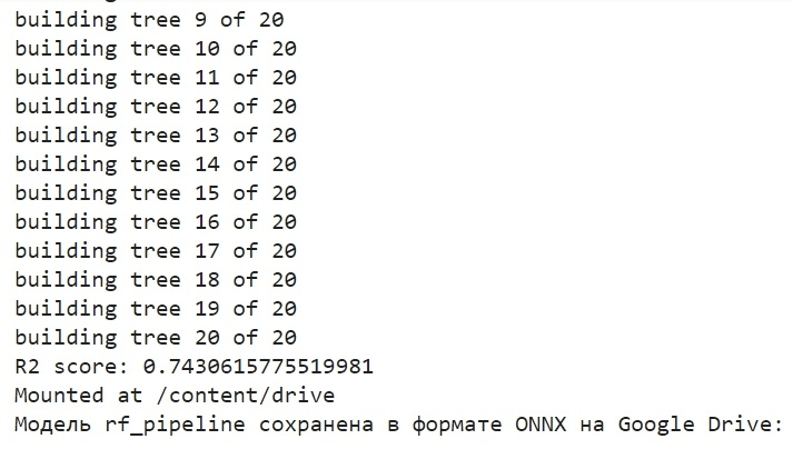
The model is saved in ONNX format to the base directory of Google Drive. ONNX can be thought of as a kind of "floppy disk" for machine learning models. This format allows you to save trained models and convert them for use in various applications. This is similar to how you save files to a flash drive and then can read them on other devices. In our case, the ONNX model will be used in the MetaTrader 5 environment to predict financial market prices. The ONNX "floppy disk" itself can be read in a third-party application, for example in MetaTrader 5. This is what we will do now.

Checking the model in the MetaTrader 5 Tester

We previously saved the ONNX model on Google Drive. Now, let's download it from there. To use this model in MetaTrader 5, let's create an Expert Advisor that will read and apply this model to make trading decisions. In the presented Expert Advisor code, set trading parameters, such as lot volume, use of stop orders, Take Profit and Stop Loss levels. Here is the code of the EA that will "read" our ONNX model:

//+------------------------------------------------------------------+
//|                                           ONNX Random Forest.mq5 |
//|                                                   Copyright 2023 |
//|                                                Evgeniy Koshtenko |
//+------------------------------------------------------------------+
#property copyright   "Copyright 2023, Evgeniy Koshtenko"
#property link        "https://www.mql5.com"
#property version     "0.90"

static vectorf ExtOutputData(1);
vectorf output_data(1);

#include <Trade\Trade.mqh>
CTrade trade;

input double InpLots       = 1.0;    // Lot volume to open a position
input bool   InpUseStops   = true;   // Trade with stop orders
input int    InpTakeProfit = 500;    // Take Profit level
input int    InpStopLoss   = 500;    // Stop Loss level
#resource "Python/rf_pipeline.onnx" as uchar ExtModel[]

#define SAMPLE_SIZE 100

long     ExtHandle=INVALID_HANDLE;
int      ExtPredictedClass=-1;
datetime ExtNextBar=0;
datetime ExtNextDay=0;
CTrade   ExtTrade;

#define PRICE_UP   1
#define PRICE_SAME 2
#define PRICE_DOWN 0

// Function for closing all positions
void CloseAll(int type=-1)
{
   for(int i=PositionsTotal()-1; i>=0; i--)
   {
      if(PositionSelectByTicket(PositionGetTicket(i)))
      {
         if(PositionGetInteger(POSITION_TYPE)==type || type==-1)
         {
            trade.PositionClose(PositionGetTicket(i));
         }
      }
   }
}

// Expert Advisor initialization
int OnInit()
{
   if(_Symbol!="EURUSD" || _Period!=PERIOD_H1)
   {
      Print("The model should work with EURUSD, H1");
      return(INIT_FAILED);
   }

   ExtHandle=OnnxCreateFromBuffer(ExtModel,ONNX_DEFAULT);
   if(ExtHandle==INVALID_HANDLE)
   {
      Print("Error creating model OnnxCreateFromBuffer ",GetLastError());
      return(INIT_FAILED);
   }

   const long input_shape[] = {1,100};
   if(!OnnxSetInputShape(ExtHandle,ONNX_DEFAULT,input_shape))
   {
      Print("Error setting the input shape OnnxSetInputShape ",GetLastError());
      return(INIT_FAILED);
   }

   const long output_shape[] = {1,1};
   if(!OnnxSetOutputShape(ExtHandle,0,output_shape))
   {
      Print("Error setting the output shape OnnxSetOutputShape ",GetLastError());
      return(INIT_FAILED);
   }

   return(INIT_SUCCEEDED);
}

// Expert Advisor deinitialization
void OnDeinit(const int reason)
{
   if(ExtHandle!=INVALID_HANDLE)
   {
      OnnxRelease(ExtHandle);
      ExtHandle=INVALID_HANDLE;
   }
}

// Process the tick function
void OnTick()
{
   if(TimeCurrent()<ExtNextBar)
      return;

   ExtNextBar=TimeCurrent();
   ExtNextBar-=ExtNextBar%PeriodSeconds();
   ExtNextBar+=PeriodSeconds();

   PredictPrice();

   if(ExtPredictedClass>=0)
      if(PositionSelect(_Symbol))
         CheckForClose();
      else
         CheckForOpen();
}

// Check position opening conditions
void CheckForOpen(void)
{
   ENUM_ORDER_TYPE signal=WRONG_VALUE;

   if(ExtPredictedClass==PRICE_DOWN)
      signal=ORDER_TYPE_SELL;
   else
   {
      if(ExtPredictedClass==PRICE_UP)
         signal=ORDER_TYPE_BUY;
   }

   if(signal!=WRONG_VALUE && TerminalInfoInteger(TERMINAL_TRADE_ALLOWED))
   {
      double price,sl=0,tp=0;
      double bid=SymbolInfoDouble(_Symbol,SYMBOL_BID);
      double ask=SymbolInfoDouble(_Symbol,SYMBOL_ASK);
      if(signal==ORDER_TYPE_SELL)
      {
         price=bid;
         if(InpUseStops)
         {
            sl=NormalizeDouble(bid+InpStopLoss*_Point,_Digits);
            tp=NormalizeDouble(ask-InpTakeProfit*_Point,_Digits);
         }
      }
      else
      {
         price=ask;
         if(InpUseStops)
         {
            sl=NormalizeDouble(ask-InpStopLoss*_Point,_Digits);
            tp=NormalizeDouble(bid+InpTakeProfit*_Point,_Digits);
         }
      }
      ExtTrade.PositionOpen(_Symbol,signal,InpLots,price,sl,tp);
   }
}

// Check position closing conditions
void CheckForClose(void)
{
   if(InpUseStops)
      return;

   bool tsignal=false;
   long type=PositionGetInteger(POSITION_TYPE);

   if(type==POSITION_TYPE_BUY && ExtPredictedClass==PRICE_DOWN)
      tsignal=true;
   if(type==POSITION_TYPE_SELL && ExtPredictedClass==PRICE_UP)
      tsignal=true;

   if(tsignal && TerminalInfoInteger(TERMINAL_TRADE_ALLOWED))
   {
      ExtTrade.PositionClose(_Symbol,3);
      CheckForOpen();
   }
}

// Function to get the current spread
double GetSpreadInPips(string symbol)
{
    double spreadPoints = SymbolInfoInteger(symbol, SYMBOL_SPREAD);
    double spreadPips = spreadPoints * _Point / _Digits;
    return spreadPips;
}

// Function to predict prices
void PredictPrice()
{
   static vectorf output_data(1);
   static vectorf x_norm(SAMPLE_SIZE);
   double spread = GetSpreadInPips(_Symbol);

   if (!x_norm.CopyRates(_Symbol, _Period, COPY_RATES_CLOSE, 1, SAMPLE_SIZE))
   {
      ExtPredictedClass = -1;
      return;
   }

   if (!OnnxRun(ExtHandle, ONNX_NO_CONVERSION, x_norm, output_data))
   {
      ExtPredictedClass = -1;
      return;
   }

   float predicted = output_data[0];

   if (spread < 0.000005 && predicted > iClose(Symbol(), PERIOD_CURRENT, 1))
   {
      ExtPredictedClass = PRICE_UP;
   }
   else if (spread < 0.000005 && predicted < iClose(Symbol(), PERIOD_CURRENT, 1))
   {
      ExtPredictedClass = PRICE_DOWN;
   }
   else
   {
      ExtPredictedClass = PRICE_SAME;
   }
}

Please pay attention that the following input dimension:

const long input_shape[] = {1,100};

must match the dimension in our Python model:

# Set the number of time steps to your requirements
n_steps = 100

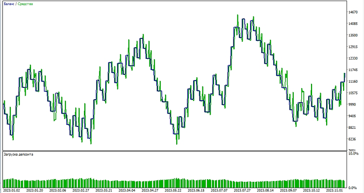
Next, we begin testing the model in the MetaTrader 5 environment. We use the model's predictions to determine the direction of price movements. If the model predicts that the price will go up, we prepare to open a long position (buy), and conversely, if the model predicts that the price will go down, we prepare to open a short position (sell). Let's test the model with a take profit of 1000 and a stop loss of 500:

Conclusion

In this article, we have considered how to create and train a Random Forest model in Python, how to preprocess data directly within the model, as well as how to export it to the ONNX standard, and then open and use the model in MetaTrader 5.

ONNX is an excellent model import-export system. It is universal and simple. Saving a model in ONNX is actually a lot easier than it looks. Data preprocessing is also very easy. 

Of course, our model of only 20 decision trees is very simple, and the random forest model itself is already a fairly old solution. In further articles, we will create more complex and modern models, using more complex data preprocessing. I would also like to note the possibility of creating an ensemble of models immediately in the form of a sklearn pipeline, simultaneously with preprocessing. This can significantly expand our capabilities, including those for classification problems.