Category Theory in MQL5 (Part 19): Naturality Square Induction

Introduction:

We have covered Category theory’s application in classifying discrete data through these article series and with quite a few examples we have shown how trading algorithms, mostly that manage trailing stops, but also those that handle entry signals as well as position sizing; can be incorporated seamlessly into an expert advisor to implement some of its concepts. MQL5 Wizard in the IDE has been instrumental in this as all shared source code needs to be assembled with the wizard to come up with a testable system.

In this article we will focus on how to utilize naturality squares, a concept we introduced in our last article, with induction. The potential applicable benefits of this will be demonstrated with 3 forex pairs that can be linked by arbitrage. We look to classify price change data for one of the pairs with the goal of assessing if we can develop an entry signal algorithm for that pair.

Naturality squares are the extension of natural transformations into a commutable diagram. So, if we have two separate categories with more than one functor between them, we can assess the relations between two or more objects in the co-domain category and use this analysis not just to relate to other similar categories but also make forecasts within the category under observation, if the objects are in a time series.

Understanding the Setup:

Our two categories for this article will have a similar structure to what we considered for the last article in that they will have two functors between them. But that will be the main similarity as in this case we will have multiple objects in both categories whereas in the last we had two objects in the domain category and only four in the codomain.

So, in the domain category that features a single time series we essentially have each price point in this series represented as an object. These ‘objects’ will be linked in their chronological order by morphisms which simply increment them to the chart timeframe the script is attached to. In addition, since we are dealing with time series, this means our category is unbound and therefore does not have a cardinality. Once again, as has been the focus in our articles, the overall size and contents of categories/ objects is not what interests us here per se but rather the morphisms and more specifically the functors from these objects.

In the codomain category we have two price time series for the other two forex pairs. Recall an arbitrage requires at least three forex pairs. They could be more but, in our case, we are using the minimum to keep our implementation relatively simple. So, the domain category will have its price series for the first pair which will be USDJPY. The two other pairs to be included in the codomain category as price series will be EURJPY, and EURUSD.

The morphisms linking the price point ‘objects’ in the second category will only be within a particular series as we do not have any linking the objects in each series at the onset.

Naturality Squares and Induction:

So, the concept of naturality squares within category theory emphasizes commutation, which in our last article was used as a means of verifying a classification. To recap if we consider the diagram below that represented four objects in the codomain category:

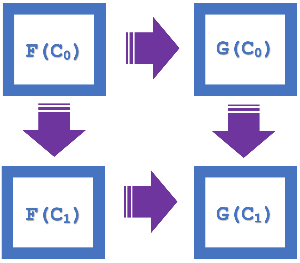
We can see there is a commutation as F(C 0 ) to G(C 0 ) and then G(C 1 ), is equivalent to F(C 0 ) to F(C 1 ) and then G(C 1 ).

The concept of induction, that is introduced for this article, highlights the ability to commute over series of multiple squares which simplifies design and saves on compute resources. If we consider the diagram below that lists n squares:

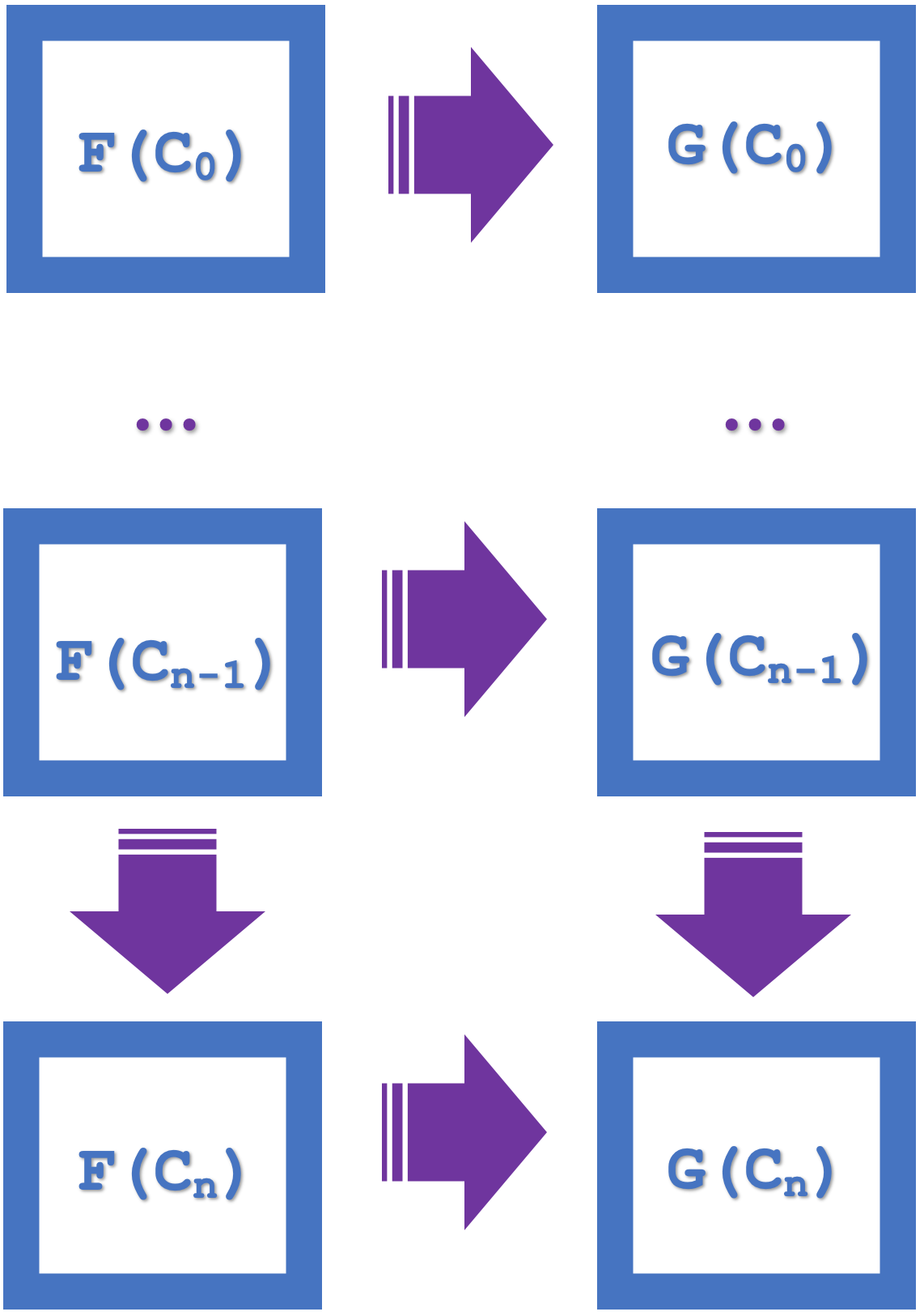
If the small naturality squares commute it follows that the larger rectangle commutes as well. This larger commutation implies morphisms and functors at an ‘n’ spacing. So, our two functors will both be from the USDJPY series but connecting to different series of EURJPY and EURUSD. The natural transformations will therefore be from EURJPY to EURUSD. Since we are using the naturality square(s) for classification as in our last article our forecasts will be for the codomain of the natural transformations’ and this is EURUSD. Induction allows us to look at these forecasts across multiple bars, as opposed to just one as we had in the last article. In the last article attempting multiple bar forecast was compute intensive given the many random decision forests that had to be employed. With induction we can now start classifying at n bars lag.

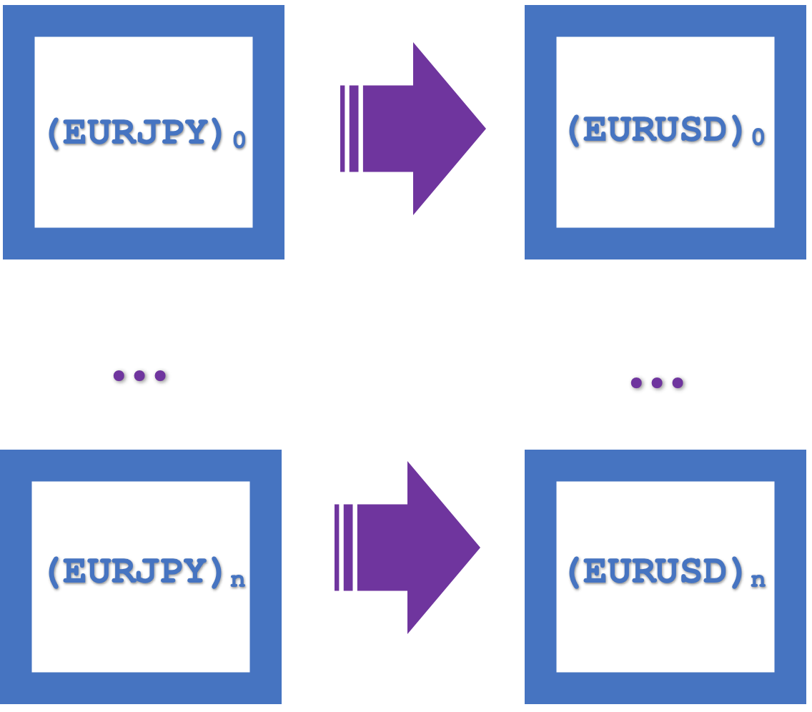
A visual representation of these naturality squares as an integrated single rectangle is shown below:

Functors role in this:

Functors have already been introduced so this paragraph serves to highlight how we are applying them with these naturality squares. In the last article we used multi-layer perceptrons to define the mapping of our functors but for this article we will look at random decision forests to serve the same purpose.

Random Decision Forests are a classifier that uses multiple learning methods (forests) to improve forecasting. Like the multi-layer perceptron (MLP), it is relatively complex, and is often referred to as an ensemble learning method. Implementing this from first principles for our purposes would be too tedious which is why it is a good thing, the Alglib already has implementation classes that are available in MQL5’s library under the ‘Include\Math’ folder.

So, the mapping by Random Decision Forests (RDFs) is defined by setting a forest size and attributing weights to the various trees & respective branches of the forest. To plainly describe them though, you could take RDFs as a team of small-decision makers where each decision maker is a tree that knows how to look at a dataset and make a choice. They all get the same question (data), and each gives an answer (decision). Once all teams have made their choice, they vote to pick the most liked decision. The cool thing about this process is even though all teams (trees) were given the same data, they each learned from different parts since they sampled randomly. Decisions from this are often smart and accurate!

I have had a go at doing my own implementation from the ground up and this algorithm, though it can be described simply, is fairly complex. Doing this with Alglib though can take a number of formats. The simplest of which only requires principally two inputs namely the number of forests, and a double type input parameter dubbed R which sets the percentage of a training set that is used to build the trees. For our purposes that is what we will use. There are other requirements like number of independent variables and number of dependent variables (aka classifiers) but these are typical to most machine learning models.

MQL5 Script Implementation:

We have strictly used MQL5’s IDE to code everything presented in these series thus far. It may be useful highlighting that besides custom indicators, expert advisors and MQL5 scripts, you can also code/ develop services, libraries, databases and even python scripts within this IDE.

For this article we are just using a script to demonstrate classification by naturality squares in induction. An expert advisor’s signal class instance would have been ideal and not just a script however implementing multi-currency signal class, though possible, is not as feasible as this article would allow therefore we will, in a non-optimized setting, print off forecast and actual changes in the close price of EURUSD and use those results to support or refute our thesis that naturality squares with induction are useful in making projections.

So, our script starts by creating an instance of the domain category to hold our series of USDJPY close price changes. This category could be used for training and is labeled as such. Although training with it would set weights for functors from it to the codomain category (our two functors), these weightings are not critical to our forecasts (as mentioned in the last article) but are mentioned here for perspective.

      //create domain series (USDJPY-rates) in first category for training
      CCategory _c_a_train;_c_a_train.Let();
      int _a_size=GetObject(_c_a_train,__currency_a,__training_start,__training_stop);

We then create an instance of the codomain category that will feature two time series as mentioned already, EURJPY and EURUSD. Since each price point represents an object, we need to take care to ‘preserve’ the two series within the category by sequentially adding the objects for each series. We are referring to them as b and c.

      //create 2 series (EURJPY and EURUSD rates) in second category for training
      CCategory _c_bc_train;_c_bc_train.Let();
      int _b_trains=GetObject(_c_bc_train,__currency_b,__training_start,__training_stop);
      int _c_trains=GetObject(_c_bc_train,__currency_c,__training_start,__training_stop);

So, our forecasts like in the last article will center on the objects in the codomain that form the naturality square. The morphisms that connect each series together with the natural transformations that link objects across series are what we will map as RDFs.

Our script has an input parameter for the number of inductions which is how we scale up the square and make projections beyond the next 1 bar. So, our naturality squares across n inductions will form a single square which we take as having the corners A, B, C, and D, such that AB and CD will be our transformations while AC and BD will be morphisms.

In implementing this mapping one can choose to use both MLPs and RDFs, say for transformations and morphisms respectively. I will leave the reader to explore that since we have seen already how MLPs can be incorporated. Moving on though we need to fill our training models for the RDF with data and this is done by matrix. The four RDFs for each mapping from AB to CD will have its own matrix and they are filled by the listing shown below:

      //create natural transformation, by induction across, n squares..., cpi to pmi
      //mapping by random forests
      int _training_size=fmin(_c_trains,_b_trains);
      int _info_ab=0,_info_bd=0,_info_ac=0,_info_cd=0;
      CDFReport _report_ab,_report_bd,_report_ac,_report_cd;
      CMatrixDouble _xy_ab;_xy_ab.Resize(_training_size,1+1);
      CMatrixDouble _xy_bd;_xy_bd.Resize(_training_size,1+1);
      CMatrixDouble _xy_ac;_xy_ac.Resize(_training_size,1+1);
      CMatrixDouble _xy_cd;_xy_cd.Resize(_training_size,1+1);
      
      double _a=0.0,_b=0.0,_c=0.0,_d=0.0;
      CElement<string> _e_a,_e_b,_e_c,_e_d;
      string _s_a="",_s_b="",_s_c="",_s_d="";
      for(int i=0;i<_training_size-__n_inductions;i++)
      {
         _s_a="";_e_a.Let();_c_bc_train.domain[i].Get(0,_e_a);_e_a.Get(1,_s_a);_a=StringToDouble(_s_a);
         _s_b="";_e_b.Let();_c_bc_train.domain[i+_b_trains].Get(0,_e_b);_e_b.Get(1,_s_b);_b=StringToDouble(_s_b);
         _s_c="";_e_c.Let();_c_bc_train.domain[i+__n_inductions].Get(0,_e_c);_e_c.Get(1,_s_c);_c=StringToDouble(_s_c);
         _s_d="";_e_d.Let();_c_bc_train.domain[i+_b_trains+__n_inductions].Get(0,_e_d);_e_d.Get(1,_s_d);_d=StringToDouble(_s_d);
         
         if(i<_training_size-__n_inductions)
         {
            _xy_ab[i].Set(0,_a);
            _xy_ab[i].Set(1,_b);
            
            _xy_bd[i].Set(0,_b);
            _xy_bd[i].Set(1,_d);
            
            _xy_ac[i].Set(0,_a);
            _xy_ac[i].Set(1,_c);
            
            _xy_cd[i].Set(0,_c);
            _xy_cd[i].Set(1,_d);
         }
      }

Once our data-sets are ready we can proceed to declare model instances for each RDF and go ahead with the individual training of each. This is done as shown below:

      CDForest          _forest;
      CDecisionForest   _rdf_ab,_rdf_cd;
      CDecisionForest   _rdf_ac,_rdf_bd;
      
      _forest.DFBuildRandomDecisionForest(_xy_ab,_training_size-__n_inductions,1,1,__training_trees,__training_r,_info_ab,_rdf_ab,_report_ab);
      _forest.DFBuildRandomDecisionForest(_xy_bd,_training_size-__n_inductions,1,1,__training_trees,__training_r,_info_bd,_rdf_bd,_report_bd);
      _forest.DFBuildRandomDecisionForest(_xy_ac,_training_size-__n_inductions,1,1,__training_trees,__training_r,_info_ac,_rdf_ac,_report_ac);
      _forest.DFBuildRandomDecisionForest(_xy_cd,_training_size-__n_inductions,1,1,__training_trees,__training_r,_info_cd,_rdf_cd,_report_cd);

The output from each training that we need to evaluate in the integer value of the ‘info’ parameter. As was the case with MLPs, this value should be positive. If all our ‘info’ parameters are positive then we can proceed with a walk forward test.

Notice our script input parameters include 3 dates namely a training start date, a training stop date, and a testing stop date. These values would ideally be validated before use to ensure they are ascending in the order I’ve stated them. Also, what is missing is a testing start date because the training stop date also acts as a testing start date. So, we implement a forward test with the listing below:

      //
      if(_info_ab>0 && _info_bd>0 && _info_ac>0 && _info_cd>0)
      {
         //create 2 objects (cpi and pmi) in second category for testing
         CCategory _c_cp_test;_c_cp_test.Let();
         int _b_test=GetObject(_c_cp_test,__currency_b,__training_stop,__testing_stop);
         ...
      
         ...
         
         MqlRates _rates[];
         ArraySetAsSeries(_rates,true);
         if(CopyRates(__currency_c,Period(), 0, _testing_size+__n_inductions+1, _rates)>=_testing_size+__n_inductions+1)
         {
            ArraySetAsSeries(_rates,true);
            
            for(int i=__n_inductions+_testing_size;i>__n_inductions;i--)
            {
               _s_a="";_e_a.Let();_c_cp_test.domain[i].Get(0,_e_a);_e_a.Get(1,_s_a);_a=StringToDouble(_s_a);
               
               double _x_ab[],_y_ab[]; ArrayResize(_x_ab,1); ArrayResize(_y_ab,1);
               ArrayInitialize(_x_ab,0.0); ArrayInitialize(_y_ab,0.0);
               //
               _x_ab[0]=_a; _forest.DFProcess(_rdf_ab,_x_ab,_y_ab);
               
               ...
               
               double _x_cd[],_y_cd[]; ArrayResize(_x_cd,1); ArrayResize(_y_cd,1);
               ArrayInitialize(_x_cd,0.0); ArrayInitialize(_y_cd,0.0);
               //
               _x_cd[0]=_y_ac[0]; _forest.DFProcess(_rdf_cd,_x_cd,_y_cd);
               
               double _c_forecast=0.0;
               if((_y_bd[0]>0.0 && _y_cd[0]>0.0)||(_y_bd[0]<0.0 && _y_cd[0]<0.0))//abd agrees with acd on currency c change
               {
                  _c_forecast=0.5*(_y_bd[0]+_y_cd[0]);
               }
               
               double _c_actual=_rates[i-__n_inductions].close-_rates[i].close;
               
               if((_c_forecast>0.0 && _c_actual>0.0)||(_c_forecast<0.0 && _c_actual<0.0)){ _strict_match++; }
               else if((_c_forecast>=0.0 && _c_actual>=0.0)||(_c_forecast<=0.0 && _c_actual<=0.0)){ _generic_match++; }
               else { _miss++; }
            }
            //
            ...
         }
      }

Remember we are interested in projecting changes to EURUSD which is represented as D in our square. In checking our projections on the forward test, we log values that strictly match in direction, values that could match in direction given that we have zeroes involved, and finally we also log the misses. This is all captured in the listing shown above.

To sum our script therefore, we start by declaring training categories, of which we critically need on for data preprocessing and training. The arbitrage forex pairs we are using are USDJPY, EURJPY, and EURUSD. We map across objects in our codomain category using RDFs that serve as morphisms in the series and natural transformations across the series to make forecasts on test data that is defined by the training stop date and the testing stop date.

Results and Analysis:

If we run the script attached at the end of this article, which implements the shared source above, we get the following logs with inductions at 1 on the daily chart of USDJPY:

2023.09.01 13:39:14.500 ct_19_r1 (USDJPY.ln,D1) void OnStart() misses: 45, strict matches: 61, & generic matches: 166, for strict pct (excl. generic): 0.58, & generic pct: 0.83, with inductions at: 1

If we however increase our inductions to 2, this is what we get:

2023.09.01 13:39:55.073 ct_19_r1 (USDJPY.ln,D1) void OnStart() misses: 56, strict matches: 63, & generic matches: 153, for strict pct (excl. generic): 0.53, & generic pct: 0.79, with inductions at: 2

There is a slight decrease, albeit a significant still a positive one, as strict matches are more than misses. We can create a log of number of inductions against matches and misses. This is shown in a graph below:

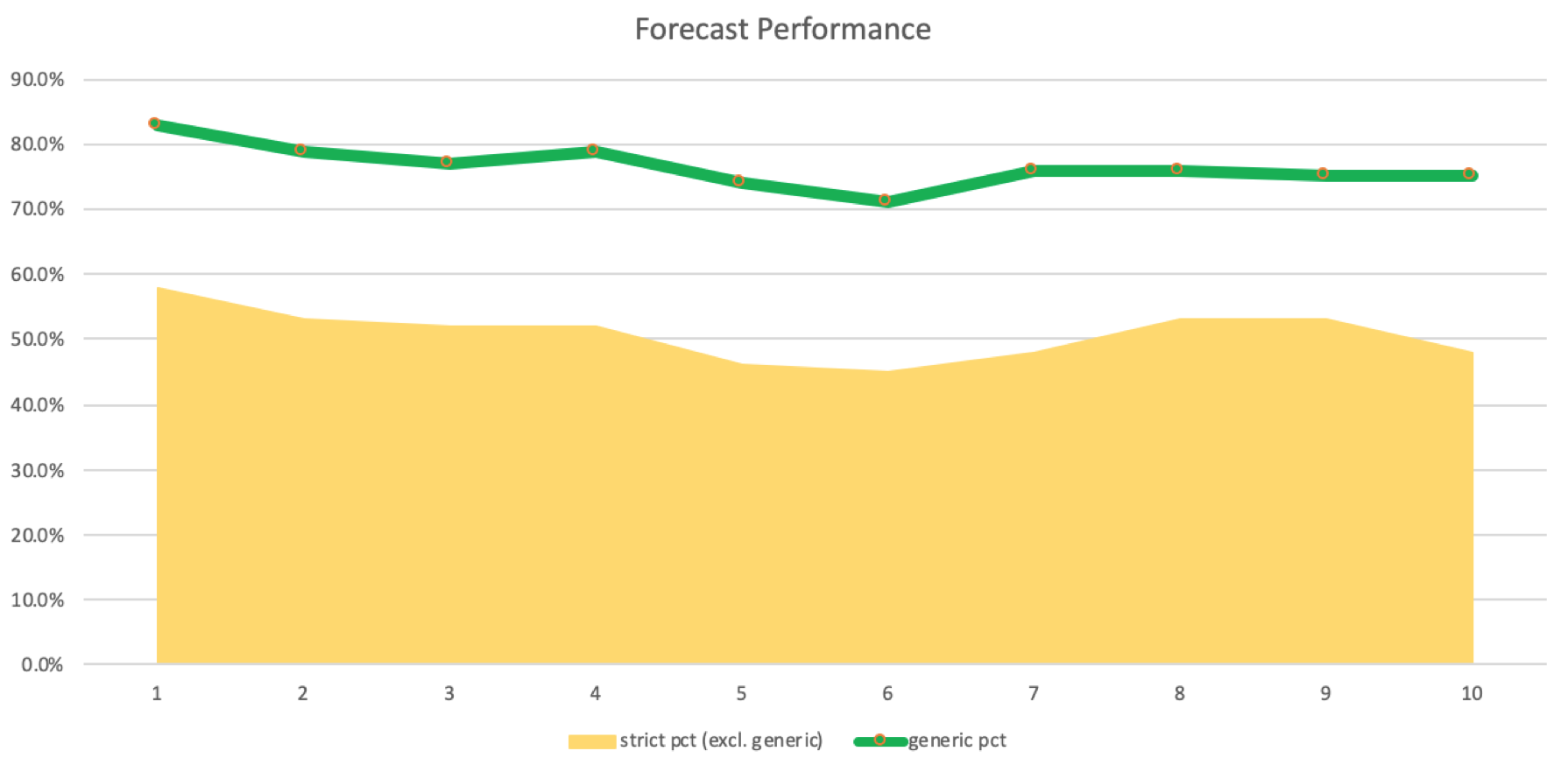
The accuracy of these forecasts and matches logged would need to be confirmed in an actual trading system that makes runs with the various induction lags to prove or disprove their performance. Quite often systems can be profitable with a smaller winning percentage meaning we cannot conclusively say using induction lags from 5 to 8 is ideal for our system. Testing with an expert advisor setup that easily accommodates multi currencies would verify this.

Main challenges faced in this implementation is inability to test as an expert signal class of an MQL5 wizard expert advisor. The wizard assembly by default initiates indicators and price buffers for one symbol only, the chart symbol. Working around this to accommodate multiple symbols is possible but requires creating a custom class that inherits from the CExpert class and making a few changes. I felt this too lengthy for this article so the reader could explore this independently.

Comparison with Traditional Methods:

Compared to ‘traditional’ methods that use simple indicators like the Moving Average our naturality square induction approach seems complex and perhaps convoluted if you were to just read its description. I do hope though that given the plethora of code libraries (such as Alglib) that are available online and in MQL5’s library the reader gets a sense of how some seemingly complex approach or idea can be easily coded in under 200 lines. Allowing one to explore, adopt or refute new ideas in a seamless manner. MQL5’s IDE is a Philomath’s paradise.

Main strengths for this system worth highlighting are its adaptability and potential accuracy.

Real-World Applications:

If we are to explore practical applications of our forecast system with arbitrage pairs, it would be within the context of trying to use arbitrage opportunities within the three pairs. Now we all know every broker has his own forex pair spread policy, and if arbitrage opportunities are to exist, it is because one of the three-pairs is mis-priced sufficiently such that the gap is more than the pair’s spread. These opportunities used to exist in years gone by but as latency has been reduced for most brokers over the years, they are quite rear. In fact, some brokers even out-law the practice.

Therefore, if we are to do arbitrage, it will be in a pseudo form where we ‘overlook’ the spread and instead look at the raw prices plus the forecast of our naturality squares. So, a simple system to go long, for instance, would look at the arbitrage price of the third pair, in our case EURUSD to be above the current quote price and the forecast to also be for a price increase. To recap the arbitrage price for EURUSD, in our case would be got by:

EURJPY / USDJPY

Incorporating such a system with what we had from the script above inevitably results in fewer trades since confirmation. for each signal is required by either a higher or lower arbitrage price for longs and shorts respectively. Working with expert signal class to produce an instance of a class that codes this is a preferred approach and since multi-currency support within the MQL5 wizard classes is not yet as robust, we can only mention it here and have the reader modify the expert class as mentioned above, or try another approach that will allow testing this multi-currency approach with wizard assembled expert advisors.

To reiterate testing ideas with MQL5 wizard made expert advisors, does not just allow putting something together with less code, it allows us to combine other exiting signals with what we are working on and to see if there is a relative weighting among the signals, that meets our results target. So for instance if rather than provide the script attached at the end, we were able to implement multi-currency and provide a workable signal file, this file could be combined with other library signal files (such as the Awesome Oscillator, RSI, etc.) or even another custom signal file by the reader, to develop a new trade system with more meaningful or balanced results than just the single signal file.

The approach of inducting naturality squares, besides potentially providing a signal file, can also be used to enhance risk-management & portfolio optimization if instead of doing a signal file, we code a custom instance of the expert money class. With this approach, though rudimentary, we could size our positions in proportion to the size of the forecast price move, with limits.

Conclusion:

To summarize key takeaways from this article, we have looked at how naturality squares when extended by induction simplify design and save on compute resources when classifying data and thus forecasts into the future.

Precise series forecasting should never be the one and end all goal of a trade system. Plenty of trade methods are sustainably profitable with a small winning percent which is why our inability to test out these ideas as an expert signal class is discouraging and clearly renders results here inconclusive on the role and potential of induction.

Thus, readers are encouraged to test further the attached code in settings that allow multi-currency support for expert advisors so as to come to better conclusions on what induction lags work and what do not.

References:

Wikipedia as per the shared links in the article.

Appendix: MQL5 Code Snippets

Attached is a script (ct_19_r1.mq5) that to be run needs to be compiled in the IDE, and then have its *.ex5 file attached to a chart in the MetaTrader 5 Terminal. It can be run with multiple settings and different arbitrage pairs beside the default ones provided. The second attached file references part category theory classes assembled this far through the series. It as always needs to be in the include folder.