
Neural networks made easy (Part 54): Using random encoder for efficient research (RE3)

Introduction
The issue of efficient exploration of the environment is one of the main problems of reinforcement learning methods. We have discussed this issue more than once. Each time, a proposed solution led to additional complication of the algorithm. In most cases, we resorted to using additional internal reward mechanisms to encourage the model to explore new actions and search for unexplored paths.
However, to assess the novelty of actions and visited states, we had to train additional models. It is important to note that the concept of "novelty of actions" does not always coincide with the completeness and uniformity of environmental research. In this aspect, methods based on estimating the entropy of actions and states look most attractive. But they impose their own limitations on the trained models. The use of entropy requires a certain understanding of the probabilities of performing actions and transitions to new states, which in the case of a continuous space of actions and states can be quite difficult for direct calculation. In search of simpler and more effective methods, I suggest you get acquainted with the Random Encoders for Efficient Exploration (RE3) algorithm presented in the article "State Entropy Maximization with Random Encoders for Efficient Exploration".
1. Main idea of RE3
Analyzing real cases with a continuous space of actions and states, we are faced with a situation where each state-action pair occurs only once in the training set. The chances of observing an identical state in the future are close to "0". The need arises to search the methods for grouping close (similar) states and actions, which leads to training additional models. For example, in the BAC method, we trained an auto encoder to evaluate the novelty of states and actions.
However, training additional models introduces some complexity into the algorithm. After all, additional time and resources are required both for selecting additional hyperparameters and for training the model. The quality of training an additional model can have a significant impact on the results of training the main Actor policy.
The main goal of the Random Encoders for Efficient Exploration (RE3) method is to minimize the number of trained models. In their work, the authors of the RE3 method draw attention to the fact that in the field of image processing, only convolutional networks are capable of identifying individual object features and characteristics. It is convolutional networks that will help reduce the dimension of multidimensional space, highlight characteristic features and cope with scaling of the original object.
The quite reasonable question here is what kind of minimization of trained models we are talking about if we additionally turn to convolutional networks?
In this aspect, the key word is "trained". The authors of the method drew attention to the fact that even a convolutional encoder initialized with random parameters effectively captures information about the proximity of two states. Below is a visualization of k-nearest states found by measuring distances in the representation space of a randomly initialized encoder (Random Encoder) and in the space of the True State from the article.

Based on this observation, the authors of the RE3 method propose to maximize the state entropy estimate in a fixed representation space of a randomly initialized encoder during model training.
The Random Encoders for Efficient Exploration (RE3) method encourages exploration in high-dimensional observation spaces by maximizing state entropy. The main idea of RE3 is to estimate entropy using the estimatork nearest neighbors in a low-dimensional space obtained using a randomly initialized encoder.
The method authors propose calculating the distance between states in the f(θ) representation space of a random encoder, whose θ parameters are randomly initialized and fixed throughout training.
The Agent's motivation arises from the observation that distances in a random encoder representation space are already useful for finding similar states without the need for representation training.
In this case, the internal reward is proportional to the assessment of the state entropy and is determined by the equation:
![]()
where yi is a state representation within the random encoder space.
In the presented internal reward equation, we use the L2 distance norm, which is always non-negative. Increasing the norm by "1" allows us to always obtain a non-negative logarithm value. Thus, we always receive a non-negative internal reward. In addition, it is easy to notice that with a sufficient number of close states, the internal reward is close to "0".
![]()
As practice shows, measuring the distance between states in a fixed representation space provides more stable internal rewards since the distance between pairs of states does not change during training.
To calculate distances in latent space, it is computationally efficient to store low-dimensional state representations in an experience replay buffer while interacting with the environment. This will eliminate the need to handle high-dimensional states through the encoder to obtain representations at each model update iteration. Moreover, this allows the distance to be calculated before all state records rather than before a single sample from a mini-batch. This scheme provides stable and accurate entropy estimation with computational efficiency.
In general, the RE3 method can be used to train an agent in real time, where the Agent learns a policy based on maximizing external rewards from the environment. Internal reward stimulates the Agent to explore the environment.
![]()
where β is a temperature ratio determining the balance between research and exploitation (β≥0).
The method authors suggest using exponential decrease for β throughout training to encourage the agent to focus more on external rewards from the environment as training progresses.
![]()
where p is a decrease rate.
While the internal reward will converge to "0" as more similar states are collected during the training, the method authors found that the decrease of β empirically stabilizes performance.
In addition, the RE3 method can be used to pre-train an Agent to explore a high-dimensional environmental space in the absence of external rewards. Subsequently, the Agent's policy can be further trained to solve specific problems.
Below is the author's visualization of the RE3 method.

The "State Entropy Maximization with Random Encoders for Efficient Exploration" article presents the results of various tests demonstrating the method efficiency. We will implement our version of the proposed algorithm and evaluate its efficiency for solving our tasks.
2. Implementation using MQL5
While we start implementing this method, it is immediately worth noting that we will not completely repeat the author’s algorithm. As always, we will use the main ideas of the method and combine them with previously considered approaches. Here we will create a certain conglomerate of the current and previously studied algorithms.
We will build our implementation based on algorithms from the Actor-Critic family. To build a convolutional encoder, we will add its description to the method for describing model architectures.
bool CreateDescriptions(CArrayObj *actor, CArrayObj *critic, CArrayObj *convolution)
  {
//---
   CLayerDescription *descr;
//---
   if(!actor)
     {
      actor = new CArrayObj();
      if(!actor)
         return false;
     }
   if(!critic)
     {
      critic = new CArrayObj();
      if(!critic)
         return false;
     }
   if(!convolution)
     {
      convolution = new CArrayObj();
      if(!convolution)
         return false;
     }
We will train a stochastic Agent policy in a continuous action space. As in previous articles, we will train the Actor using algorithms from the Actor-Critic family. Since we will use the approaches of the RE3 method to estimate the entropy component of the reward, we can simplify the Actor model. In this case, we will re-create the Actor architecture from the article "Behavior-Guided Actor-Critic".
//--- Actor
   actor.Clear();
//--- Input layer
   if(!(descr = new CLayerDescription()))
      return false;
   descr.type = defNeuronBaseOCL;
   int prev_count = descr.count = (HistoryBars * BarDescr);
   descr.activation = None;
   descr.optimization = ADAM;
   if(!actor.Add(descr))
     {
      delete descr;
      return false;
     }
//--- layer 1
   if(!(descr = new CLayerDescription()))
      return false;
   descr.type = defNeuronBatchNormOCL;
   descr.count = prev_count;
   descr.batch = 1000;
   descr.activation = None;
   descr.optimization = ADAM;
   if(!actor.Add(descr))
     {
      delete descr;
      return false;
     }
//--- layer 2
   if(!(descr = new CLayerDescription()))
      return false;
   descr.type = defNeuronConvOCL;
   prev_count = descr.count = prev_count - 1;
   descr.window = 2;
   descr.step = 1;
   descr.window_out = 8;
   descr.activation = LReLU;
   descr.optimization = ADAM;
   if(!actor.Add(descr))
     {
      delete descr;
      return false;
     }
//--- layer 3
   if(!(descr = new CLayerDescription()))
      return false;
   descr.type = defNeuronConvOCL;
   prev_count = descr.count = prev_count;
   descr.window = 8;
   descr.step = 8;
   descr.window_out = 8;
   descr.activation = LReLU;
   descr.optimization = ADAM;
   if(!actor.Add(descr))
     {
      delete descr;
      return false;
     }
//--- layer 4
   if(!(descr = new CLayerDescription()))
      return false;
   descr.type = defNeuronBaseOCL;
   descr.count = 256;
   descr.optimization = ADAM;
   descr.activation = LReLU;
   if(!actor.Add(descr))
     {
      delete descr;
      return false;
     }
//--- layer 5
   if(!(descr = new CLayerDescription()))
      return false;
   descr.type = defNeuronBaseOCL;
   prev_count = descr.count = 128;
   descr.activation = LReLU;
   descr.optimization = ADAM;
   if(!actor.Add(descr))
     {
      delete descr;
      return false;
     }
//--- layer 6
   if(!(descr = new CLayerDescription()))
      return false;
   descr.type = defNeuronConcatenate;
   descr.count = LatentCount;
   descr.window = prev_count;
   descr.step = AccountDescr;
   descr.optimization = ADAM;
   descr.activation = SIGMOID;
   if(!actor.Add(descr))
     {
      delete descr;
      return false;
     }
//--- layer 7
   if(!(descr = new CLayerDescription()))
      return false;
   descr.type = defNeuronBaseOCL;
   descr.count = 256;
   descr.activation = LReLU;
   descr.optimization = ADAM;
   if(!actor.Add(descr))
     {
      delete descr;
      return false;
     }
//--- layer 8
   if(!(descr = new CLayerDescription()))
      return false;
   descr.type = defNeuronBaseOCL;
   descr.count = 256;
   descr.activation = LReLU;
   descr.optimization = ADAM;
   if(!actor.Add(descr))
     {
      delete descr;
      return false;
     }
//--- layer 9
   if(!(descr = new CLayerDescription()))
      return false;
   descr.type = defNeuronBaseOCL;
   descr.count = 2 * NActions;
   descr.activation = LReLU;
   descr.optimization = ADAM;
   if(!actor.Add(descr))
     {
      delete descr;
      return false;
     }
//--- layer 10
   if(!(descr = new CLayerDescription()))
      return false;
   descr.type = defNeuronVAEOCL;
   descr.count = NActions;
   descr.optimization = ADAM;
   if(!actor.Add(descr))
     {
      delete descr;
      return false;
     }
As before, our Critic will not have the block of preliminary processing of source data. We will use the latent state of our Actor as the critic's input. We will also use reward decomposition, while slightly reducing the number of reward points. Instead of 6 separate elements of entropy components for each action, we will have only one element of internal reward.
//+------------------------------------------------------------------+
//| Rewards structure                                                |
//|   0     -  Delta Balance                                         |
//|   1     -  Delta Equity ( "-" Drawdown / "+" Profit)             |
//|   2     -  Penalty for no open positions                         |
//|   3     -  Mean distance                                         |
//+------------------------------------------------------------------+
As a result, we get the following Critic architecture.
//--- Critic
   critic.Clear();
//--- Input layer
   if(!(descr = new CLayerDescription()))
      return false;
   descr.type = defNeuronBaseOCL;
   prev_count = descr.count = LatentCount;
   descr.activation = None;
   descr.optimization = ADAM;
   if(!critic.Add(descr))
     {
      delete descr;
      return false;
     }
//--- layer 1
   if(!(descr = new CLayerDescription()))
      return false;
   descr.type = defNeuronConcatenate;
   descr.count = LatentCount;
   descr.window = prev_count;
   descr.step = NActions;
   descr.optimization = ADAM;
   descr.activation = LReLU;
   if(!critic.Add(descr))
     {
      delete descr;
      return false;
     }
//--- layer 2
   if(!(descr = new CLayerDescription()))
      return false;
   descr.type = defNeuronBaseOCL;
   descr.count = LatentCount;
   descr.activation = LReLU;
   descr.optimization = ADAM;
   if(!critic.Add(descr))
     {
      delete descr;
      return false;
     }
//--- layer 3
   if(!(descr = new CLayerDescription()))
      return false;
   descr.type = defNeuronBaseOCL;
   descr.count = LatentCount;
   descr.activation = LReLU;
   descr.optimization = ADAM;
   if(!critic.Add(descr))
     {
      delete descr;
      return false;
     }
//--- layer 4
   if(!(descr = new CLayerDescription()))
      return false;
   descr.type = defNeuronBaseOCL;
   descr.count = NRewards;
   descr.optimization = ADAM;
   descr.activation = None;
   if(!critic.Add(descr))
     {
      delete descr;
      return false;
     }
Next we have to describe the architecture of the convolutional encoder. Here is the first difference from the described method. The RE3 method provides an internal reward based on an estimate of the distance between latent state representations. In contrast, we will use a latent representation of "state-action" pairs reflected in the size of the encoder source data layer.
//--- Convolution
   convolution.Clear();
//--- Input layer
   if(!(descr = new CLayerDescription()))
      return false;
   descr.type = defNeuronBaseOCL;
   prev_count = descr.count = (HistoryBars * BarDescr) + AccountDescr + NActions;
   descr.activation = None;
   descr.optimization = ADAM;
   if(!convolution.Add(descr))
     {
      delete descr;
      return false;
     }
Our encoder model is not trained and there is no point in using a batch data normalization layer. But we will use a fully connected layer and at its output we will obtain comparable data that can be processed by convolutional layers.
//--- layer 1
   if(!(descr = new CLayerDescription()))
      return false;
   descr.type = defNeuronBaseOCL;
   descr.count = 512;
   descr.window = prev_count;
   descr.step = NActions;
   descr.optimization = ADAM;
   descr.activation = SIGMOID;
   if(!convolution.Add(descr))
     {по
      delete descr;
      return false;
     }
Then we reduce the dimensionality of the data using 3 successive convolutional layers. Their task is to determine characteristic features for identifying similar states and actions.
//--- layer 2
   if(!(descr = new CLayerDescription()))
      return false;
   descr.type = defNeuronConvOCL;
   prev_count = descr.count = 512 / 8;
   descr.window = 8;
   descr.step = 8;
   int prev_wout = descr.window_out = 2;
   descr.activation = LReLU;
   descr.optimization = ADAM;
   if(!convolution.Add(descr))
     {
      delete descr;
      return false;
     }
//--- layer 3
   if(!(descr = new CLayerDescription()))
      return false;
   descr.type = defNeuronConvOCL;
   prev_count = descr.count = (prev_count * prev_wout) / 4;
   descr.window = 4;
   descr.step = 4;
   prev_wout = descr.window_out = 2;
   descr.activation = LReLU;
   descr.optimization = ADAM;
   if(!convolution.Add(descr))
     {
      delete descr;
      return false;
     }
//--- layer 4
   if(!(descr = new CLayerDescription()))
      return false;
   descr.type = defNeuronConvOCL;
   prev_count = descr.count = (prev_count * prev_wout) / 4;
   descr.window = 4;
   descr.step = 4;
   prev_wout = descr.window_out = 2;
   descr.activation = LReLU;
   descr.optimization = ADAM;
   if(!convolution.Add(descr))
     {
      delete descr;
      return false;
     }
To complete the encoder, we will use a fully connected layer and reduce the hidden representation of the data to a given dimension.
//--- layer 5
   if(!(descr = new CLayerDescription()))
      return false;
   descr.type = defNeuronBaseOCL;
   descr.count = EmbeddingSize;
   descr.activation = LReLU;
   descr.optimization = ADAM;
   if(!convolution.Add(descr))
     {
      delete descr;
      return false;
     }
//---
   return true;
  }
Please note that we used LReLU in all neural layers (except the first one) to activate neurons. The absence of limits to the range of results of the activation function will allow the objects to be divided into groups as accurately as possible.
After creating descriptions of our models' architecture, let's talk a little about the experience replay buffer. The method authors propose to simultaneously save a latent representation of the state into the experience playback buffer along with the standard data set. I agree with that. It is quite logical to calculate the latent representation of the state once and subsequently use it in the training process without the need for recalculation at each iteration.
In our sequence of actions, when we first launch the training data collection EA "...\RE3\Research.mq5", there are no pre-trained models saved yet. The Actor model is created by the EA and filled with random parameters. We can also generate a random encoder model. But parallel launch of several EA instances in the optimization mode of the strategy tester will create an encoder for each EA pass. The problem is that in each pass we will get a random encoder, whose latent representation will not be comparable with similar representations in other passes. This completely violates the ideas and principles of the RE3 method.
I see two possible solutions:
- preliminary creation and saving of models before the first launch of the "...\RE3\Research.mq5" EA
- generating an encoder and encoding representations in the body of the "...\RE3\Study.mq5" model training EA.
I chose the second option in my implementation. Therefore, we will not make changes to the data storage structures and the "...\RE3\Research.mq5" training sample collection EA. You can find its full code in the attachment.
Next we move on to working on the "...\RE3\Study.mq5" model training EA. Here we create objects for 6 models, while we will train only 3 of them. For target models, we apply soft updating of parameters using the ꚍ ratio.
CNet                 Actor;
CNet                 Critic1;
CNet                 Critic2;
CNet                 TargetCritic1;
CNet                 TargetCritic2;
CNet                 Convolution;
In the EA initialization method, we load the training set and pre-trained models. If the models cannot be loaded, then we generate new models filled with random parameters.
int OnInit()
  {
//---
   ResetLastError();
   if(!LoadTotalBase())
     {
      PrintFormat("Error of load study data: %d", GetLastError());
      return INIT_FAILED;
     }
//--- load models
   float temp;
   if(!Actor.Load(FileName + "Act.nnw", temp, temp, temp, dtStudied, true) ||
      !Critic1.Load(FileName + "Crt1.nnw", temp, temp, temp, dtStudied, true) ||
      !Critic2.Load(FileName + "Crt2.nnw", temp, temp, temp, dtStudied, true) ||
      !Convolution.Load(FileName + "CNN.nnw", temp, temp, temp, dtStudied, true) ||
      !TargetCritic1.Load(FileName + "Crt1.nnw", temp, temp, temp, dtStudied, true) ||
      !TargetCritic2.Load(FileName + "Crt2.nnw", temp, temp, temp, dtStudied, true))
     {
      CArrayObj *actor = new CArrayObj();
      CArrayObj *critic = new CArrayObj();
      CArrayObj *convolution = new CArrayObj();
      if(!CreateDescriptions(actor, critic, convolution))
        {
         delete actor;
         delete critic;
         delete convolution;
         return INIT_FAILED;
        }
      if(!Actor.Create(actor) || !Critic1.Create(critic) || !Critic2.Create(critic) ||
         !Convolution.Create(convolution))
        {
         delete actor;
         delete critic;
         delete convolution;
         return INIT_FAILED;
        }
      if(!TargetCritic1.Create(critic) || !TargetCritic2.Create(critic))
        {
         delete actor;
         delete critic;
         delete convolution;
         return INIT_FAILED;
        }
      delete actor;
      delete critic;
      delete convolution;
      //---
      TargetCritic1.WeightsUpdate(GetPointer(Critic1), 1.0f);
      TargetCritic2.WeightsUpdate(GetPointer(Critic2), 1.0f);
      StartTargetIter = StartTargetIteration;
     }
   else
      StartTargetIter = 0;
As in the previous article, when generating new models, we extend the time to use the target models. This allows us to pre-train target models before using them to estimate subsequent Agent states and actions.
Here we transfer all models into a single OpenCL context.
//---
   OpenCL = Actor.GetOpenCL();
   Critic1.SetOpenCL(OpenCL);
   Critic2.SetOpenCL(OpenCL);
   TargetCritic1.SetOpenCL(OpenCL);
   TargetCritic2.SetOpenCL(OpenCL);
   Convolution.SetOpenCL(OpenCL);
Before the training, we check the compliance of the architectures of the models used.
   Actor.getResults(Result);
   if(Result.Total() != NActions)
     {
      PrintFormat("The scope of the actor does not match the actions count (%d <> %d)", NActions, Result.Total());
      return INIT_FAILED;
     }
//---
   Actor.GetLayerOutput(0, Result);
   if(Result.Total() != (HistoryBars * BarDescr))
     {
      PrintFormat("Input size of Actor doesn't match state description (%d <> %d)", Result.Total(),
                                                                                        (HistoryBars * BarDescr));
      return INIT_FAILED;
     }
//---
   Actor.GetLayerOutput(LatentLayer, Result);
   int latent_state = Result.Total();
   Critic1.GetLayerOutput(0, Result);
   if(Result.Total() != latent_state)
     {
      PrintFormat("Input size of Critic doesn't match latent state Actor (%d <> %d)", Result.Total(), latent_state);
      return INIT_FAILED;
     }
At the end of the method, we create an auxiliary buffer and generate a model training event.
   Gradient.BufferInit(AccountDescr, 0);
//---
   if(!EventChartCustom(ChartID(), 1, 0, 0, "Init"))
     {
      PrintFormat("Error of create study event: %d", GetLastError());
      return INIT_FAILED;
     }
//---
   return(INIT_SUCCEEDED);
  }
In the EA deinitialization method, we update the parameters of the target models and save the training results.
void OnDeinit(const int reason)
  {
//---
   TargetCritic1.WeightsUpdate(GetPointer(Critic1), Tau);
   TargetCritic2.WeightsUpdate(GetPointer(Critic2), Tau);
   Actor.Save(FileName + "Act.nnw", 0, 0, 0, TimeCurrent(), true);
   TargetCritic1.Save(FileName + "Crt1.nnw", Critic1.getRecentAverageError(), 0, 0, TimeCurrent(), true);
   TargetCritic2.Save(FileName + "Crt2.nnw", Critic2.getRecentAverageError(), 0, 0, TimeCurrent(), true);
   Convolution.Save(FileName + "CNN.nnw", 0, 0, 0, TimeCurrent(), true);
   delete Result;
  }
The actual process of training models is organized in the Train procedure. But here its algorithm will be slightly different from similar procedures of the previously considered EAs.
First, we will count the total number of states in the training set. As you know, the number of states in each individual pass is stored in the Total variable. We will arrange a loop and collect the total sum of the values of the specified variable from each pass.
void Train(void)
  {
   int total_tr = ArraySize(Buffer);
   uint ticks = GetTickCount();
//---
   int total_states = Buffer[0].Total;
   for(int i = 1; i < total_tr; i++)
      total_states += Buffer[i].Total;
We need the resulting value to declare matrices of a compressed representation of state-action pairs and the collected actual rewards from the environment.
   vector<float> temp;
   Convolution.getResults(temp);
   matrix<float> state_embedding = matrix<float>::Zeros(total_states,temp.Size());
   matrix<float> rewards = matrix<float>::Zeros(total_states,NRewards);
Next, we will arrange a loop system, in which we will create latent representations for all state-action pairs from the training set. Here we first collect the original data into a single data buffer.
   for(int tr = 0; tr < total_tr; tr++)
     {
      for(int st = 0; st < Buffer[tr].Total; st++)
        {
         State.AssignArray(Buffer[tr].States[st].state);
         float PrevBalance = Buffer[tr].States[MathMax(st,0)].account[0];
         float PrevEquity = Buffer[tr].States[MathMax(st,0)].account[1];
         State.Add((Buffer[tr].States[st].account[0] - PrevBalance) / PrevBalance);
         State.Add(Buffer[tr].States[st].account[1] / PrevBalance);
         State.Add((Buffer[tr].States[st].account[1] - PrevEquity) / PrevEquity);
         State.Add(Buffer[tr].States[st].account[2]);
         State.Add(Buffer[tr].States[st].account[3]);
         State.Add(Buffer[tr].States[st].account[4] / PrevBalance);
         State.Add(Buffer[tr].States[st].account[5] / PrevBalance);
         State.Add(Buffer[tr].States[st].account[6] / PrevBalance);
         double x = (double)Buffer[tr].States[st].account[7] / (double)(D'2024.01.01' - D'2023.01.01');
         State.Add((float)MathSin(x != 0 ? 2.0 * M_PI * x : 0));
         x = (double)Buffer[tr].States[st].account[7] / (double)PeriodSeconds(PERIOD_MN1);
         State.Add((float)MathCos(x != 0 ? 2.0 * M_PI * x : 0));
         x = (double)Buffer[tr].States[st].account[7] / (double)PeriodSeconds(PERIOD_W1);
         State.Add((float)MathSin(x != 0 ? 2.0 * M_PI * x : 0));
         x = (double)Buffer[tr].States[st].account[7] / (double)PeriodSeconds(PERIOD_D1);
         State.Add((float)MathSin(x != 0 ? 2.0 * M_PI * x : 0));
         State.AddArray(Buffer[tr].States[st].action);
Then we call the forward pass of the convolutional encoder.
         if(!Convolution.feedForward(GetPointer(State),1,false,NULL))
           {
            PrintFormat("%s -> %d", __FUNCTION__, __LINE__);
            ExpertRemove();
            return;
           }
The obtained result is saved in the corresponding row of the state and action embedding matrix. We save the corresponding external reward into the reward matrix with the same string number. After that, increase the counter of recorded lines.
         Convolution.getResults(temp);
         state_embedding.Row(temp,state);
         temp.Assign(Buffer[tr].States[st].rewards);
         rewards.Row(temp,state);
         state++;
The time spent on this process depends on the size of the training sample and can be significant. Therefore, in the loop body, we will add the information message to get the visual control of the process.
         if(GetTickCount() - ticks > 500)
           {
            string str = StringFormat("%-15s %6.2f%%", "Embedding ", state * 100.0 / (double)(total_states));
            Comment(str);
            ticks = GetTickCount();
           }
        }
     }
Once the loop system iterations are complete, we will adjust the matrix sizes to the number of rows stored.
   if(state != total_states)
     {
      rewards.Resize(state,NRewards);
      state_embedding.Reshape(state,state_embedding.Cols());
      total_states = state;
     }
This concludes the preparatory stage. It is time to move directly to training the models. Here, as before, we arrange a training cycle with the number of iterations specified by the user in the EA external parameters.
   vector<float> rewards1, rewards2;
   for(int iter = 0; (iter < Iterations && !IsStopped()); iter ++)
     {
      int tr = (int)((MathRand() / 32767.0) * (total_tr - 1));
      int i = (int)((MathRand() * MathRand() / MathPow(32767, 2)) * (Buffer[tr].Total - 2));
      if(i < 0)
        {
         iter--;
         continue;
        }
In the loop body, we randomly select a pass and state for the current iteration of model training. Then we check the need to use the target models.
If our training process has reached the threshold of using target models, then we generate post-state inputs for a forward pass through those models.
      vector<float> reward, target_reward = vector<float>::Zeros(NRewards);
      reward.Assign(Buffer[tr].States[i].rewards);
      //--- Target
      if(iter >= StartTargetIter)
        {
         State.AssignArray(Buffer[tr].States[i + 1].state);
         float PrevBalance = Buffer[tr].States[i].account[0];
         float PrevEquity = Buffer[tr].States[i].account[1];
         Account.Clear();
         Account.Add((Buffer[tr].States[i + 1].account[0] - PrevBalance) / PrevBalance);
         Account.Add(Buffer[tr].States[i + 1].account[1] / PrevBalance);
         Account.Add((Buffer[tr].States[i + 1].account[1] - PrevEquity) / PrevEquity);
         Account.Add(Buffer[tr].States[i + 1].account[2]);
         Account.Add(Buffer[tr].States[i + 1].account[3]);
         Account.Add(Buffer[tr].States[i + 1].account[4] / PrevBalance);
         Account.Add(Buffer[tr].States[i + 1].account[5] / PrevBalance);
         Account.Add(Buffer[tr].States[i + 1].account[6] / PrevBalance);
         double x = (double)Buffer[tr].States[i + 1].account[7] / (double)(D'2024.01.01' - D'2023.01.01');
         Account.Add((float)MathSin(x != 0 ? 2.0 * M_PI * x : 0));
         x = (double)Buffer[tr].States[i + 1].account[7] / (double)PeriodSeconds(PERIOD_MN1);
         Account.Add((float)MathCos(x != 0 ? 2.0 * M_PI * x : 0));
         x = (double)Buffer[tr].States[i + 1].account[7] / (double)PeriodSeconds(PERIOD_W1);
         Account.Add((float)MathSin(x != 0 ? 2.0 * M_PI * x : 0));
         x = (double)Buffer[tr].States[i + 1].account[7] / (double)PeriodSeconds(PERIOD_D1);
         Account.Add((float)MathSin(x != 0 ? 2.0 * M_PI * x : 0));
         //---
         if(Account.GetIndex() >= 0)
            Account.BufferWrite();
We remember that we need a description of the initial state of the environment and the actions of the Agent for direct pass of the target models of Critics. Here there are two points we need a direct pass of the Actor for:
- Critics do not have a pre-processing unit for the source data (they do not use a latent representation of the Actor);
- The target model of the Critic evaluates the subsequent state in the light of using the current Actor policy (generation of a new vector of actions is necessary).
Therefore, we first perform a forward Actor pass.
         if(!Actor.feedForward(GetPointer(State), 1, false, GetPointer(Account)))
           {
            PrintFormat("%s -> %d", __FUNCTION__, __LINE__);
            break;
           }
Then we call the methods of direct passage of two models of target Critics.
         if(!TargetCritic1.feedForward(GetPointer(Actor), LatentLayer, GetPointer(Actor)) ||
            !TargetCritic2.feedForward(GetPointer(Actor), LatentLayer, GetPointer(Actor)))
           {
            PrintFormat("%s -> %d", __FUNCTION__, __LINE__);
            break;
           }
Next, in accordance with the Soft Actor-Critic algorithm, we need to select a target model with a minimum estimate of the subsequent state. In my implementation, I used a simple summation of reward elements. But if your model provides different weighting ratios for individual elements of the reward function, then you can use the vector product of the model results and the vector of weighting ratios.
         TargetCritic1.getResults(rewards1);
         TargetCritic2.getResults(rewards2);
         if(rewards1.Sum() <= rewards2.Sum())
            target_reward = rewards1;
         else
            target_reward = rewards2;
We then subtract the actual reward received from interacting with the environment from the predicted results of the selected model and adjust for the discount factor.
         for(ulong r = 0; r < target_reward.Size(); r++)
            target_reward -= Buffer[tr].States[i + 1].rewards[r];
         target_reward *= DiscFactor;
        }
Thus, in the target_reward vector, we obtained the variance for each reward item between the Critic's predicted score and the actual reward from the environment. How can this be of help?
As you might remember, the experience replay buffer for each "state-action" pair stores the cumulative amount of reward until the end of the passage taking into account the discount factor. This total reward is accumulated based on the policies used by the Agent while interacting with the environment.
We predicted the cost of the "state-action" pair above taking into account the current policy of the Agent and subtracted the estimate of the same state while considering the action from the experience replay buffer. Thus, the target_reward vector now features the effect of the Actor's policy change on the state value.
Note that we are talking about a change in the state value. After all, it practically does not depend on the Agent. However, its actions in the same state may differ depending on the policy used.
After assessing the impact of changing the Actor’s action policy on the overall result, we move on to the Critics training block. It is the quality of their training that affects the correctness of passing the error gradient to the Actor’s actions.
Here we also prepare environmental description data, which includes historical data of price movements and indicators. We also prepare account status data as a separate buffer.
      //--- Q-function study
      State.AssignArray(Buffer[tr].States[i].state);
      float PrevBalance = Buffer[tr].States[MathMax(i - 1, 0)].account[0];
      float PrevEquity = Buffer[tr].States[MathMax(i - 1, 0)].account[1];
      Account.Clear();
      Account.Add((Buffer[tr].States[i].account[0] - PrevBalance) / PrevBalance);
      Account.Add(Buffer[tr].States[i].account[1] / PrevBalance);
      Account.Add((Buffer[tr].States[i].account[1] - PrevEquity) / PrevEquity);
      Account.Add(Buffer[tr].States[i].account[2]);
      Account.Add(Buffer[tr].States[i].account[3]);
      Account.Add(Buffer[tr].States[i].account[4] / PrevBalance);
      Account.Add(Buffer[tr].States[i].account[5] / PrevBalance);
      Account.Add(Buffer[tr].States[i].account[6] / PrevBalance);
      double x = (double)Buffer[tr].States[i].account[7] / (double)(D'2024.01.01' - D'2023.01.01');
      Account.Add((float)MathSin(x != 0 ? 2.0 * M_PI * x : 0));
      x = (double)Buffer[tr].States[i].account[7] / (double)PeriodSeconds(PERIOD_MN1);
      Account.Add((float)MathCos(x != 0 ? 2.0 * M_PI * x : 0));
      x = (double)Buffer[tr].States[i].account[7] / (double)PeriodSeconds(PERIOD_W1);
      Account.Add((float)MathSin(x != 0 ? 2.0 * M_PI * x : 0));
      x = (double)Buffer[tr].States[i].account[7] / (double)PeriodSeconds(PERIOD_D1);
      Account.Add((float)MathSin(x != 0 ? 2.0 * M_PI * x : 0));
      if(Account.GetIndex() >= 0)
         Account.BufferWrite();
Once the data preparation work is complete, we perform a forward Actor pass.
      if(!Actor.feedForward(GetPointer(State), 1, false, GetPointer(Account)))
        {
         PrintFormat("%s -> %d", __FUNCTION__, __LINE__);
         break;
        }
However, this time we take only a latent representation of the environment state from the Actor. We use the Agent's action from the experience playback buffer. After all, it is precisely for this action that we have actual reward from the environment.
Using this data, we carry out a direct pass of both Critics.
      Actions.AssignArray(Buffer[tr].States[i].action);
      if(Actions.GetIndex() >= 0)
         Actions.BufferWrite();
      //---
      if(!Critic1.feedForward(GetPointer(Actor), LatentLayer, GetPointer(Actions)) ||
         !Critic2.feedForward(GetPointer(Actor), LatentLayer, GetPointer(Actions)))
        {
         PrintFormat("%s -> %d", __FUNCTION__, __LINE__);
         break;
        }
Next, we need to generate target values and perform a reverse pass of the Critics. We have already performed similar operations several times. Typically, at this stage, we would adjust the actual reward from the experience replay buffer to the effect of the changed policy and pass the resulting value as a target value to both Critic models. But we use decomposed reward in this implementation. In the previous article, we used the Conflict-Averse Gradient Descent (CAGrad) algorithm to correct the error gradient. We corrected the deviation of values in the CNet_SAC_D_DICE::CAGrad method and saved the obtained values directly into the error gradient buffer of the neural results layer. Currently, we do not have the ability to directly access the gradient buffer of the last neural layer of the models and we need target values.
Let's perform a little data manipulation to obtain target values corrected using the Conflict-Averse Gradient Descent method. First, we generate target values from the available data. Then we subtract the Critic’s predicted values from them, thereby obtaining a deviation (error). Let's correct the resulting deviation using the already familiar CAGrad method. Add the predicted value of the Critic, which we subtracted earlier, to the result.
This gives us a target value adjusted using the Conflict-Averse Gradient Descent method. However, such a target value is only relevant for one Critic model. For the second model of the Critic, we will have to repeat the operations considering its predicted values.
After performing the Critics backpass, we perform a partial Actor backpass to distribute the error gradient across the data preprocessing block.
      Critic1.getResults(rewards1);
      Result.AssignArray(CAGrad(reward + target_reward - rewards1) + rewards1);
      if(!Critic1.backProp(Result, GetPointer(Actions), GetPointer(Gradient)) ||
         !Actor.backPropGradient(GetPointer(Account), GetPointer(Gradient), LatentLayer))
        {
         PrintFormat("%s -> %d", __FUNCTION__, __LINE__);
         break;
        }
      Critic2.getResults(rewards2);
      Result.AssignArray(CAGrad(reward + target_reward - rewards2) + rewards2);
      if(!Critic2.backProp(Result, GetPointer(Actions), GetPointer(Gradient)) ||
         !Actor.backPropGradient(GetPointer(Account), GetPointer(Gradient), LatentLayer))
        {
         PrintFormat("%s -> %d", __FUNCTION__, __LINE__);
         break;
        }
Updating the Critics' parameters is followed by the Actor policy update block. In accordance with the Soft Actor-Critic algorithm, a Critic with a minimum state estimate is used to update the Actor parameters. We will use a Critic with the minimum average error, which will potentially yield a more correct transmission of the error gradient.
      //--- Policy study
      CNet *critic = NULL;
      if(Critic1.getRecentAverageError() <= Critic2.getRecentAverageError())
         critic = GetPointer(Critic1);
      else
         critic = GetPointer(Critic2);
Here we introduce the RE3 method into our training process. We collect into a single data buffer descriptions of the analyzed state of the environment, the state of the account and the selected action of the agent, taking into account the updated policy. Let me remind you that we carried out a direct pass of the Actor at the stage of updating the Critics' parameters.
After that, carry out a direct pass of the selected Critic. This time we evaluate the actions of the Actor in the analyzed state taking into account the updated policy. Call a direct pass of our Encoder to obtain an embedding of the pair of the analyzed state and the Actor’s action with the updated policy.
      Actor.getResults(rewards1);
      State.AddArray(GetPointer(Account));
      State.AddArray(rewards1);
      if(!critic.feedForward(GetPointer(Actor), LatentLayer, GetPointer(Actor)) ||
         !Convolution.feedForward(GetPointer(State)))
        {
         PrintFormat("%s -> %d", __FUNCTION__, __LINE__);
         break;
        }
The forward pass is followed by a reverse pass of the models. So we again have to form the Critic’s target values. But this time we have to combine the CAGrad and RE3 algorithms. In addition, we do not have the correct target values for the analyzed state and the Actor action with the updated policy.
We have moved the definition of the target value using RE3 approaches into a separate KNNReward function. We will have a look at its algorithm a bit little later. The adjustment of the decomposed reward is carried out according to the algorithm described in the Critics' parameters update block.
      Convolution.getResults(rewards1);
      critic.getResults(reward);
      reward += CAGrad(KNNReward(7,rewards1,state_embedding,rewards) - reward);
      //---
      Result.AssignArray(reward + target_reward);
Next, we just have to disable the Critic’s training mode and sequentially call the backpass methods for the Critic and the Actor. Also, we should not forget to check the results of the operations.
      critic.TrainMode(false);
      if(!critic.backProp(Result, GetPointer(Actor)) ||
         !Actor.backPropGradient(GetPointer(Account), GetPointer(Gradient)))
        {
         PrintFormat("%s -> %d", __FUNCTION__, __LINE__);
         critic.TrainMode(true);
         break;
        }
      critic.TrainMode(true);
After updating the Actor policy, we return the Critic to the model training mode.
At the end of the model training cycle, we update the parameters of the target models and inform a user about the training progress.
      //--- Update Target Nets
      TargetCritic1.WeightsUpdate(GetPointer(Critic1), Tau);
      TargetCritic2.WeightsUpdate(GetPointer(Critic2), Tau);
      //---
      if(GetTickCount() - ticks > 500)
        {
         string str = StringFormat("%-15s %5.2f%% -> Error %15.8f\n", "Critic1",
                                     iter * 100.0 / (double)(Iterations), Critic1.getRecentAverageError());
         str += StringFormat("%-15s %5.2f%% -> Error %15.8f\n", "Critic2",
                                     iter * 100.0 / (double)(Iterations), Critic2.getRecentAverageError());
         Comment(str);
         ticks = GetTickCount();
        }
     }
After completing all iterations of the model training process, we clear the comments field, display the training results to the log and initiate EA termination.
   Comment("");
//---
   PrintFormat("%s -> %d -> %-15s %10.7f", __FUNCTION__, __LINE__, "Critic1", Critic1.getRecentAverageError());
   PrintFormat("%s -> %d -> %-15s %10.7f", __FUNCTION__, __LINE__, "Critic2", Critic2.getRecentAverageError());
   ExpertRemove();
//---
  }
We have already considered the algorithm of the Train model training method. In order to fully understand the process, it is necessary to analyze the algorithm of the CAGrad and KNNReward functions. The algorithm of the first one is completely transferred from the method of the same name, discussed in the previousarticle. You can find it in the attachment. I suggest focusing on the second function algorithm. Moreover, it differs from the original algorithm described above.
In its parameters, the KNNReward function receives the number of neighbors to analyze, the embedding vector of the desired state, the state embedding matrix from the training set and the reward matrix. Let me remind you that the state embedding matrices from the experience and reward playback buffer are synchronized by rows. We will exploit this important point later.
The result of the function operations is returned as a vector of values of the corresponding rewards.
vector<float> KNNReward(ulong k, vector<float> &embedding, matrix<float> &state_embedding, matrix<float> &rewards)
  {
   if(embedding.Size() != state_embedding.Cols())
     {
      PrintFormat("%s -> %d Inconsistent embedding size", __FUNCTION__, __LINE__);
      return vector<float>::Zeros(0);
     }
In the function body, we first check the size of the embedding of the analyzed state and the created embeddings of the experience playback buffer.
Next, we determine the distance between the embedding vectors. To do this, we subtract the value of the corresponding element of the description of the analyzed state from each embedding column of the states of the experience playback buffer. Square the resulting values.
   ulong size = embedding.Size();
   ulong states = state_embedding.Rows();
   ulong rew_size = rewards.Cols();
   matrix<float> temp = matrix<float>::Zeros(states,size);
//---
   for(ulong i = 0; i < size; i++)
      temp.Col(MathPow(state_embedding.Col(i) - embedding[i],2.0f),i);
Extract the square root of the row-by-row sum and place the resulting vector in the first column of the matrix.
temp.Col(MathSqrt(temp.Sum(1)),0);
Thus, we have obtained the distances between the desired state and examples from the experience reproduction buffer in the first column of our matrix.
Let's change the dimension of our matrix and add the corresponding reward elements from the experience playback buffer to the adjacent columns.
   temp.Resize(states,1 + rew_size);
   for(ulong i = 0; i < rew_size; i++)
      temp.Col(rewards.Col(i),i + 1);
As a result of these operations, we received a reward matrix whose first column contains the distance to the desired state in the compressed embedding space.
As you might remember, in this case, the desired state is the analyzed state with the Actor’s action according to the updated policy.
Now, in order to determine the internal reward for a given Actor action, we need to determine k nearest neighbors. It is quite logical that we can easily find them after sorting the resulting matrix in descending order of distances. However, to completely sort the values, we will need several successive passes over the entire distance vector. At the same time, we do not need to completely sort the matrix. Our task is to find only k minimum values. Their sequence in the small matrix of results is not too important to us. Thus, we only need one pass along the distance vector.
We only copy k first rows to our results matrix. Determine the maximum distance and the position of the maximum distance element in the small matrix. Next, arrange a cycle of searching through the remaining rows of the original matrix. In the body of the loop, we sequentially check the distance to the analyzed state and the maximum one in our result matrix. If we find a closer state, we store it in the maximum distance row of our result matrix. Then we update the value of the maximum distance and its position in the matrix of minimum distances.
   matrix<float> min_dist = temp;
   min_dist.Resize(k,rew_size + 1);
   float max = min_dist.Col(0).Max();
   ulong max_row = min_dist.Col(0).ArgMax();
   for(ulong i = k; i < states; i++)
     {
      if(temp[i,0] >= max)
         continue;
      min_dist.Row(temp.Row(i),max_row);
      max = min_dist.Col(0).Max();
      max_row = min_dist.Col(0).ArgMax();
     }
Repeat iterations until all rows of our matrix of distances and rewards are completely enumerated. After one complete search in the min_dist minimum distance matrix, we get k minimum distances (k nearest neighbors) with corresponding rewards from the experience replay buffer. They may not be sorted, but we do not need this to calculate the internal reward.
   vector<float> t = vector<float>::Ones(k);
   vector<float> ri = MathLog(min_dist.Col(0) + 1.0f);
At this stage, we have all the data to determine the internal reward (entropy) of the action being analyzed. But we still have an open question about the target value of the reward for the analyzed state and action. Here it is worth paying attention once again to the obtained k nearest neighbors. After all, we have attached the appropriate rewards to them. Our entire process of training models is based on statistics of states-actions and received rewards. Hence, k-nearest neighbors are our representative sample and the relevance of their rewards for the desired action is directly proportional to the embedding distance.
Thus, we define the target reward as the distance-weighted average of the reward from the k-nearest neighbors.
   t = (t - ri) / k;
//---
   vector<float> result = vector<float>::Zeros(rew_size);
   for(ulong i = 0; i < rew_size - 1; i++)
      result[i] = (t * min_dist.Col(i + 1)).Sum();
In the field of the entropy component of the reward function, we write the average value as the logarithm of distances using the RE3 method.
   result[rew_size - 1] = ri.Mean();
//---
   return (result);
  }
We have fully defined the vector of decomposed reward target values and return the vector of results to the calling program.
This concludes our review of the methods and functions of the "...\RE3\Study.mq5" model training EA. The complete code of this EA and all programs used in the article can be found in the attachment.
3. Test
The implementation presented above can probably hardly be called the Random Encoders for Efficient Exploration (RE3) method in its pure form. However, we used the basic approaches of this algorithm and supplemented them with our vision of previously studied algorithms. The time has come to evaluate the results using real historical data.
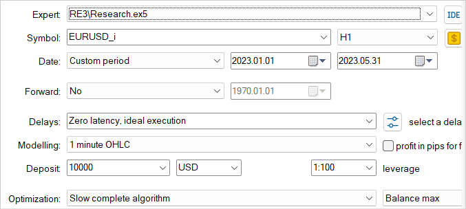
As before, training and testing of models is carried out on the first 5 months of 2023 of EURUSD H1. All indicator parameters are used by default. The initial balance is USD 10,000.
Let me repeat once again that training models is an iterative process. First, we launch the EA in the strategy tester for interaction with the "...\RE3\Research.mq5" environment and collecting training examples.
Here we use a slow optimization mode with exhaustive search of parameters, which allows us to fill the experience playback buffer with the most diverse data. This provides the broadest possible understanding of the nature of the model environment.
The collected training examples are used by the "...\RE3\Study.mq5" model training EA while training Critics and Actor.
We repeat the iterations of collecting training examples and training models several times until the desired result is obtained.
While preparing the article, I was able to train an Actor policy capable of generating profit on the training set. On the training set, the EA showed an impressive 83% of profitable trades. Although I should admit that the number of trades performed is very small. During the 5 months of the training period, my Actor made only 6 trades. Only one of them was closed with a relatively small loss of USD 18.62. The average profitable trade is USD 114.96. As a result, the profit factor exceeded 30, while the recovery factor amounted to 4.62.


Based on the testing results, we can conclude that the proposed algorithm makes it possible to find effective combinations. However, 5.5% profitability and 6 trading operations in 5 months is a rather low result. To achieve better results, we should focus on increasing the number of performed trades. However, keep in mind that an increase in the number of operations does not lead to a deterioration in the overall strategy efficiency.
Conclusion
In this article, we introduced the Random Encoders for Efficient Exploration (RE3) method, which is an efficient approach to exploring the environment in the context of reinforcement learning. This method aims to solve the problem of efficiently exploring complex environments, which is one of the main challenges in the field of deep reinforcement learning.
The main idea of RE3 is to estimate the entropy of states in the space of low-dimensional representations obtained using a randomly initialized encoder. The encoder parameters are fixed throughout training. This avoids introducing additional models and training representations, which makes the method simpler and computationally efficient.
In the practical part of the article, I presented my vision and implementation of the proposed method. My implementation uses the basic ideas of the proposed algorithm, but is supplemented by a number of approaches from previously considered algorithms. This made it possible to create and train a rather interesting model. The share of profitable trades is pretty amazing, but unfortunately the total number of trades is very small.
In general, the resulting model has potential, but additional work is required to find ways to increase the number of trades.
Links
- State Entropy Maximization with Random Encoders for Efficient Exploration
- Neural networks made easy (Part 51): Behavior-Guided Actor-Critic (BAC)
- Neural networks made easy (Part 53): Reward decomposition
Programs used in the article
| # | Name | Type | Description |
|---|---|---|---|
| 1 | Research.mq5 | Expert Advisor | Example collection EA |
| 2 | Study.mq5 | Expert Advisor | Agent training EA |
| 3 | Test.mq5 | Expert Advisor | Model testing EA |
| 4 | Trajectory.mqh | Class library | System state description structure |
| 5 | NeuroNet.mqh | Class library | A library of classes for creating a neural network |
| 6 | NeuroNet.cl | Code Base | OpenCL program code library |
Translated from Russian by MetaQuotes Ltd.
Original article: https://www.mql5.com/ru/articles/13158
Warning: All rights to these materials are reserved by MetaQuotes Ltd. Copying or reprinting of these materials in whole or in part is prohibited.
This article was written by a user of the site and reflects their personal views. MetaQuotes Ltd is not responsible for the accuracy of the information presented, nor for any consequences resulting from the use of the solutions, strategies or recommendations described.

 How to create a simple Multi-Currency Expert Advisor using MQL5 (Part 5): Bollinger Bands On Keltner Channel — Indicators Signal
- Free trading apps
- Over 8,000 signals for copying
- Economic news for exploring financial markets
You agree to website policy and terms of use
Dmtry__1.PNG (1916×320) (mql5.com)