
Modified Grid-Hedge EA in MQL5 (Part I): Making a Simple Hedge EA

Introduction
Are you looking to dive into the world of trading with Expert Advisors (EAs) but keep bumping into this line - "No dangerous Hedging/Grid/Martingale used"? You might wonder what's all the fuss about these strategies. Why do people keep saying they're risky, and what's the real deal behind these claims? Maybe you're even thinking, "Hey, can we tweak these strategies to make them safer?" Plus, why do traders bother with these strategies in the first place? What's good and bad about them? If these thoughts have crossed your mind, you're in the right place. Your search for answers is about to end. We'll start by creating a simple hedge Expert Advisor. Think of it as the first step towards our bigger project - a Grid-Hedge Expert Advisor. This will be a cool mix of the classic grid and hedge strategies. By the end of this article, you'll know how to whip up a basic hedge strategy and get the lowdown on whether this strategy is as profitable as some say. But we're not stopping there. Throughout this series, we'll explore these strategies inside out. We'll figure out what works, what doesn’t, and how we can mix and match to make something even better. Our goal? To see if we can take these traditional strategies, give them a fresh twist, and use them to make some solid profit with automated trading. So, stick with me, and let's find out together!Here's a quick overview of what we'll tackle in this article:
- Discussing the Classic Hedge Strategy
- Automation of Classic Hedge Strategy
- Backtesting our Classic Hedge Strategy
- Conclusion
Discussing the Classic Hedge Strategy
First and foremost, we should discuss the strategy before going further.
First, we open a buy position, say for simplicity, at a 1000 price level and put the stop loss at 950, and take the profit at 1050. That is, if we hit the stop loss, we lose $50, and if we hit the take profit, we gain $50. Now we hit take profit, strategy ends here, and we go home with a profit. But in case it hits stop loss, we will lose $50. Now what we do is place a sell position immediately at 950 and set take profit at 900 and stop loss at 1000. If this new sell position hits take profit, ... we gain $50 but the catch is we already lost $50 so our net gain is $0 and in case it hits stop loss that is price level 1000, we again lose $50 so our total loss is $100, but now at this point we again place a buy position with the same take profit and stop loss as the previous buy position. In case this new buy position hits TP, we get $50 and our total net gain is -$50-$50+$50 = -$50, that is a loss of $50 and in case it hits stop loss, our total is -$50-$50-$50=-$150, that is a total loss of $150.
For simplicity, we are ignoring the spreads, and commissions for now.
Now you might be thinking, "What is happening here, and how will we get 100% like this?" But you are missing one major thing: lot size. What if we increase the lot size of consecutive positions? So now, let's review our strategy.
We open a buy position of 0.01 lot (minimum possible) at 1000:
- if we hit take profit (1050), we go home with profit of $50 and strategy ends here.
- if we hit stop loss (950), we lose $50.
If we hit stop loss then strategy doesn't end according to the above rule. According to our strategy we will immediately place a sell position of 0.02 (doubled) lot size at 950:
- If we hit take profit (900), we will gain total net profit of -$50+$100 = $50 and strategy ends here.
- if we hit stop loss (1000), we will lose $50+$100 = $150 in total.
If we hit stop loss then strategy doesn't end according to the above rule. According to our strategy we will immediately place a buy position of 0.04 (again doubled) lot size at 1000:
- if we hit take profit (1050), we will gain total net profit of -$50-$100+$200 = $50 and strategy ends here.
- if we hit stop loss (950), we will lose $50+$100+$150=$350 in total.
If we hit stop loss then strategy doesn't end according to the above rule. According to our strategy we will immediately place a sell position of 0.08 (again doubled) lot size at 950:
- If we hit take profit (900), we will gain total net profit of -$50-$100-$150+$400 = $50 and strategy ends here.
- if we hit stop loss (1000), we will lose $50+$100+$150+$200 = $500 in total.
...
As you might have already noticed, in any case we are getting a profit of $50 when the strategy ends. If not, then the strategy continues. This strategy will continue until we hit take profit at either 900 or 1050; price will eventually hit either of these two points, and we will get a guaranteed $50 profit for sure.
In the above case, we placed a buy position first, but it is not mandatory to start with a buy position. Alternatively, we can start the strategy with a sell position of 0.01 (in our case).
Actually, this alternative of starting with a sell position is very important as we will be modifying the strategy later on so that we get as much flexibility as possible, like for example we might need to define an entry point (initial buy in our case) for the above cycle, but restricting that entry point to buy position only will be problematic as we might define the entry point such that it will be beneficial to place a sell position initially.
The strategy starting with sell position will be exactly symmetric to the above case of starting with buy position. Just to explain this more clearly, our strategy will look something like this:
- if we hit take profit (900), we go home with profit of $50 and strategy ends here.
- if we hit stop loss (1000), we lose $50.
If we hit stop loss then strategy doesn't end according to the above rule. According to our strategy we will immediately place a buy position of 0.02 (doubled) lot size at 1000:
- If we hit take profit (1050), we will gain total net profit of -$50+$100 = $50 and strategy ends here.
- if we hit stop loss (950), we will lose $50+$100 = $150 in total.
If we hit stop loss then strategy doesn't end according to the above rule. According to our strategy we will immediately place a sell position of 0.04 (doubled again) lot size at 950:
- if we hit take profit (900), we will gain total net profit of -$50-$100+$200 = $50 and strategy ends here.
- if we hit stop loss (1000), we will lose $50+$100+$150 = $350 in total.
... and so on.
Again, as we can see, this strategy ends only when we hit either the 900 or 1050 price levels, leading to a profit of $50 for sure. If we do not hit those price levels, the strategy continues until we eventually reach them.
Note: It is not mandatory to increase the lot size by a factor of 2. We can increase it by any factor, although any multiplier less than 2 will not guarantee a profit for both of the above cases. We chose 2 for simplicity and may potentially change this while optimizing the strategy later on.
So, that concludes our discussion of the Classic Hedge Startegy.
Dicussing Automation of our Classic Hedge Startegy
First, we need to discuss the plan for how we will proceed with creating an Expert Advisor. Actually, there are quite a lot of approaches to do this. Two major approaches are as follows:
- Approach #1: Defining four levels (variables) as stated by the strategy and placing positions whenever these lines are crossed by the price again as stated by our strategy.
- Approach #2: Using pending orders and detecting when that pending order is executed and place further pending orders when that happens.
Both approaches are almost equivalent, and it is debatable which one is slightly better, but I will discuss only Approach #1 as it is easier to code and understand.
Automation of Classic Hedge Strategy
First, We will declare few variables in global space:
input bool initialPositionBuy = true;
input double buyTP = 15;
input double sellTP = 15;
input double buySellDiff = 15;
input double initialLotSize = 0.01;
input double lotSizeMultiplier = 2;
- isPositionBuy is bool variable which will be deciding which position type will be placed next i.e. buy position or sell position. if it is true, next position type will be Buy and Sell otherwise.
- buyTP is the distance between A and B that is the take profit of buy positions (in pips), where A, B will be defined later on.
- sellTP is the distance between C and D that is the take profit of sell positions (in pips), where C, D will be defined later on.
- buySellDiff is the distance between B and C that is buy price level and sell price level (in pips).
- intialLotSize is the Lot Size of the first position.
- lotSizeMultiplier is the multiplier of the lot size for consecutive position.
Note: These variables will be used later to optimize the strategy.
For instance, We put buyTP, sellTP and buySellDiff equal to 15 pips but we will be changing these later on and see what values give us optimal profit and drawdown.
These are the input variables that later on will be used for optimization.
Now, We create some more variables in global space:
double A, B, C, D;
bool isPositionBuy;
bool hedgeCycleRunning = false;
double lastPositionLotSize;
- We first defined 4 levels named A, B, C, D as double variables:
- A: This represents the price level of the take profit for all the buy positions.
- B: This represents the opening price level for all the buy position and stop loss of all the sell positions.
- C: This represents the opening price level for all the sell position and stop loss of all the buy positions.
- D: This represents the price level of the take profit for all the sell positions.
- isPositionBuy: This is a bool variable which can take 2 values, true and false where true represents that the initial position is buy and false represents that the initial position is sell.
- hedgeCycleRunning: This is a bool variable which can again take 2 values, true and false where true represents that one hedge cycle is running that is that the initial order has been opened but A or D price levels that we defined above have not been reached yet while false represents that price level has reached either A or D and new cycle will then be started which we will see later. Also, this variable will be false by default.
- lastPositionLotSize: As the name suggests, this double type variable always contains the lot size of the last opened order and in case cycle has not been started, it will take the value equal to the input variable initialLotSize which we will set later.
//+------------------------------------------------------------------+
//| Hedge Cycle Intialization Function                               |
//+------------------------------------------------------------------+
void StartHedgeCycle()
   {
    isPositionBuy = initialPositionBuy;
    double initialPrice = isPositionBuy ? SymbolInfoDouble(_Symbol, SYMBOL_ASK) : SymbolInfoDouble(_Symbol, SYMBOL_BID);
    A = isPositionBuy ? initialPrice + buyTP * _Point * 10 : initialPrice + (buySellDiff + buyTP) * _Point * 10;
    B = isPositionBuy ? initialPrice : initialPrice + buySellDiff * _Point * 10;
    C = isPositionBuy ? initialPrice - buySellDiff * _Point * 10 : initialPrice;
    D = isPositionBuy ? initialPrice - (buySellDiff + sellTP) * _Point * 10 : initialPrice - sellTP * _Point * 10;

    ObjectCreate(0, "A", OBJ_HLINE, 0, 0, A);
    ObjectSetInteger(0, "A", OBJPROP_COLOR, clrGreen);
    ObjectCreate(0, "B", OBJ_HLINE, 0, 0, B);
    ObjectSetInteger(0, "B", OBJPROP_COLOR, clrGreen);
    ObjectCreate(0, "C", OBJ_HLINE, 0, 0, C);
    ObjectSetInteger(0, "C", OBJPROP_COLOR, clrGreen);
    ObjectCreate(0, "D", OBJ_HLINE, 0, 0, D);
    ObjectSetInteger(0, "D", OBJPROP_COLOR, clrGreen);

    ENUM_ORDER_TYPE positionType = isPositionBuy ? ORDER_TYPE_BUY : ORDER_TYPE_SELL;
    double SL = isPositionBuy ? C : B;
    double TP = isPositionBuy ? A : D;
    CTrade trade;
    trade.PositionOpen(_Symbol, positionType, initialLotSize, initialPrice, SL, TP);

    lastPositionLotSize = initialLotSize;
    if(trade.ResultRetcode() == 10009) hedgeCycleRunning = true;
    isPositionBuy = isPositionBuy ? false : true;
   }
//+------------------------------------------------------------------+
The function type is void, meaning we don't need it to return anything. The function works as follows:
First, we set the isPositionBuy variable (bool) equal to the input variable initialPositionBuy, which will tell us which position type to place at the start of each cycle. You might be wondering why we need two variables if they are both the same, but note that we will be changing isPositionBuy alternatively (last line of the above code block). However, initialPositionBuy is always fixed and we do not change it.
Then we define a new variable (double type) named initialPrice which we set equal to Ask or Bid using a ternary operator. If isPositionBuy is true, then initialPrice becomes equal to the Ask Price at that point in time, and Bid Price otherwise.
Then we define the variables (double type) that we discussed earlier briefly i.e. A, B, C, D variables using ternary operator as follows:
- If isPositionBuy is True:
- A equals to sum of initialPrice and buyTP (input variable) where buyTP is multiplied by the factor of (_Point*10), where _Point is actually the predefined function "Point()".
- B equals to initialPrice
- C equals initialPrice minus buySellDiff (input variable) where buySellDiff is multiplied by the factor of (_Point*10).
- D equals initialPrice minus sum of buySellDiff and sellTP which is multiplied by the factor of (_Point*10).
- If isPositionBuy is False:
- A equals to sum of initialPrice and (buySellDiff + buyTP) which is multiplied by the factor of (_Point*10).
- B equals to sum of initialPrice and buySellDiff where buySellDiff is multiplied by a factor of (_Point*10).
- C equals to initialPrice
- D equals initialPrice minus sellTP where sellTP is multiplied by the factor of (_Point*10).
Now, for visualization, we draw some lines on the chart representing A, B, C, D price levels using ObjectCreate and set their color property to clrGreen using ObjectSetInteger (you can use any other colour also).
Now we need to open the initial order that can be buy or sell depending on the variable isPositionBuy. Now to do that we define three variables: positionType, SL, TP.
- positionType: The type of this variable is ENUM_ORDER _TYPE which is a predefined custom variable type that can take integer values from 0 to 8 according to the following table:
Integer Values Identifier 0 ORDER_TYPE_BUY 1 ORDER_TYPE_SELL 2 ORDER_TYPE_BUY_LIMIT 3 ORDER_TYPE_SELL_LIMIT 4 ORDER_TYPE_BUY_STOP 5 ORDER_TYPE_SELL_STOP 6 ORDER_TYPE_BUY_STOP_LIMIT 7 ORDER_TYPE_SELL_STOP_LIMIT 8 ORDER_TYPE_CLOSE_BY As you can see that 0 represents ORDER_TYPE_BUY and 1 represents ORDER_TYPE_SELL, we only need these two. We will be using Identifier rather than integer values as they are hard to remember.
-
SL: if isPositionBuy is true then SL equals price level C otherwise it equals B
-
TP: if isPositionBuy is true then TP equals price level A otherwise it equals D
Using these 3 variables, we need place a position as follow:
First we import the standard trade library using #include:
#include <Trade/Trade.mqh>
Now, just before opening the position, we create a instance of the CTrade class using:
CTrade trade;
trade.PositionOpen(_Symbol, positionType, initialLotSize, initialPrice, SL, TP); And using that instance we place a position with PositionOpen function in that instance with following parameters:
- _Symbol gives current symbol that the Expert Advisor is attached to.
- positionType is the ENUM_ORDER_TYPE variable we defined earlier.
- initial lot size is the input variable.
- initialPrice is the order opening price which is either Ask (for buy positions) or Bid (for sell positions).
- Finally we provide SL and TP price levels.
With that a Buy or Sell position will be placed. Now, After the position is place, we store it's Lot Size in the variable defined in global space named lastPositionLotSize so that we can use this lot and multiplier from input to calculate lot size of further position.
With that we are left with 2 more things to do:
if(trade.ResultRetcode() == 10009) hedgeCycleRunning = true;
isPositionBuy = isPositionBuy ? false : true;
Here, we set the value of hedgeCycleRunning to true only when a position is placed successfully. This is determined by the ResultRetcode() function in the CTrade instance named trade, which returns "10009" indicating a successful placement (you can see all these return codes here). The reason for using hedgeCycleRunning will be explained by further code.
One last thing is we're using the ternary operator to alternate the value of isPositionBuy. If it was false, it will become true and vice versa. We do this because our strategy states that once an initial position is opened, a sell will be placed after a buy and a buy will be placed after a sell, meaning it alternates.
This concludes our discussion of our fundamentally important function StartHedgeCycle(), as we will be using this function again and again.
Now, let's proceed with our final piece of code.
//+------------------------------------------------------------------+
//| Expert tick function                                             |
//+------------------------------------------------------------------+
void OnTick()
   {
    double _Ask = SymbolInfoDouble(_Symbol, SYMBOL_ASK);
    double _Bid = SymbolInfoDouble(_Symbol, SYMBOL_BID);

    if(!hedgeCycleRunning)
       {
        StartHedgeCycle();
       }

    if(_Bid <= C && !isPositionBuy)
       {
        double newPositionLotSize = NormalizeDouble(lastPositionLotSize * lotSizeMultiplier, 2);
        trade.PositionOpen(_Symbol, ORDER_TYPE_SELL, newPositionLotSize, _Bid, B, D);
        lastPositionLotSize = newPositionLotSize;
        isPositionBuy = isPositionBuy ? false : true;
       }

    if(_Ask >= B && isPositionBuy)
       {
        double newPositionLotSize = NormalizeDouble(lastPositionLotSize * lotSizeMultiplier, 2);
        trade.PositionOpen(_Symbol, ORDER_TYPE_BUY, newPositionLotSize, _Ask, C, A);
        lastPositionLotSize = newPositionLotSize;
        isPositionBuy = isPositionBuy ? false : true;
       }

    if(_Bid >= A || _Ask <= D)
       {
        hedgeCycleRunning = false;
       }
   }
//+------------------------------------------------------------------+
First two lines are self-explanatory, they just define _Ask and _Bid (double variables) that store Ask and Bid at that point in time.
Then we use an if-statement to start the hedge cycle using the StartHedgeCycle() function if the hedgeCycleRunning variable is false. We already know what the StartHedgeCycle() function does, but to summarize, it does the following:
- Define A, B, C, D price levels.
- Draw horizontal green lines on A, B, C, D price levels for visualization.
- Open a position.
- Store this position's Lot Size in lastPositionLotSize variable defined in global space so that it can be used everywhere.
- Set hedgeCycleRunning to true as it was false before that is exactly why we executed StartHedgeCycle() function.
- Finally, alternate the isPositionBuy variable from true to false and false to true as stated by our strategy.
We only execute StartHedgeCycle() once because we executed it if hedgeCycleRunning was false, and at the end of the function, we change it to false. Therefore, unless we set hedgeCycleRunning to false again, StartHedgeCycle() will not be executed again.
Let's skip the next two if-statements for now, and we will come back to them later. Let's see the final if-statement:
if(_Bid >= A || _Ask <= D)
   {
    hedgeCycleRunning = false;
   }
This handles the restarting of the cycle. As we discussed earlier, if we set hedgeCycleRunning to true, the cycle will restart and everything we discussed previously will happen again. In addition, I have ensured that when the cycle restarts, all positions from the previous cycle will be closed with either take profit (whether it is a Buy or Sell position).
So, we handled cycle start, cycle end, and restart, but we are still missing the main part, which is handling the order opening when the price hits B level from below or C level from above. The position type must also be alternative, where Buy only opens at B level and Sell only opens at C level.
We skipped the code that handles this, so let's get back to it.
if(_Bid <= C && !isPositionBuy)
   {
    double newPositionLotSize = NormalizeDouble(lastPositionLotSize * lotSizeMultiplier, 2);
    CTrade trade;
    trade.PositionOpen(_Symbol, ORDER_TYPE_SELL, newPositionLotSize, _Bid, B, D);
    lastPositionLotSize = lastPositionLotSize * lotSizeMultiplier;
    isPositionBuy = isPositionBuy ? false : true;
   }

if(_Ask >= B && isPositionBuy)
   {
    double newPositionLotSize = NormalizeDouble(lastPositionLotSize * lotSizeMultiplier, 2);
    CTrade trade;
    trade.PositionOpen(_Symbol, ORDER_TYPE_BUY, newPositionLotSize, _Ask, C, A);
    lastPositionLotSize = lastPositionLotSize * lotSizeMultiplier;
    isPositionBuy = isPositionBuy ? false : true;
   }
So, these two if statements handle the order opens in between the cycle (between the initial position being placed and cycle not ending yet).
- First IF-Statement: This handles opening a sell order. If the Bid variable (which contains the Bid price at that point in time) is below or equal to the C level and isPositionBuy is false, then we define a double variable called newPositionLotSize. This is set equal to lastPositionLotSize multiplied by the lotSizeMultiplier, and then the double value is normalized up to 2 decimal places using a predefined function called NormalizeDouble.
Then, we place a sell position using the predefined function PositionOpen() from the CTrade instance named trade, giving the newPositionLotSize as a parameter. Finally, we set lastPositionLotSize to this new lot size (without normalization) so that we can multiply it in further positions, and at last, we alternate the isPositionBuy from true to false or false to true. - Second IF statement: This handles opening a buy order. If the Ask price (variable containing the Ask price at that point in time) is equal to or above the B level and isPositionBuy is true, then we define a double variable named newPositionLotSize. We set newPositionLotSize equal to lastPositionLotSize multiplied by lotSizeMultiplier and normalize the double value up to two decimal places using the predefined function NormalizeDouble, as before.
Then, we place a buying position using the predefined function PositionOpen() from the CTrade instance named trade, giving the newPositionLotSize as a parameter. Finally, we set lastPositionLotSize to this new lot size (without normalization) so that we can multiply it in further positions. Lastly, we alternate the isPositionBuy from true to false or false to true.
There are 2 very important points to take note of here:
-
In the first IF statement, we used "Bid" price and stated to open a position when "Bid" goes below or equal to "C" and "isBuyPosition" is false. Why did we use "Bid" here?
Suppose we use the Ask price, then there is a possibility that the previous buy position is closed, but the new sell position doesn't get opened. This is because we know that the buy opens at Ask and closes at Bid, leaving a possibility that the buy will be closed when Bid crosses or equals the C price level line from above. This will close the buy order by the stop loss we set earlier while opening the position, but the sell is not opened yet. So, if the price that is ask and bid both goes up, then our strategy was not being followed through. That is the reason we used Bid instead of Ask.Symmetrically, in the second IF statement, we used the Ask price and stated that we would open a position when Ask goes above or equals B and isBuyPosition is true. Why did we use Ask here?
Suppose we use Bid price, then there is a possibility that the previous sell position is closed, but the new buy position is not opened. We know that the sell opens at Bid and closes at Ask, which leaves a possibility that the sell will be closed when Ask crosses or equals the B price level line from below, thus closing the sell order by the stop loss we set earlier while opening the position. However, the buy is not opened yet. So, if the price that Ask and Bid both go down, then our strategy was not being followed through. That is why we used Ask instead of Bid.
So, the whole point is that if a Buy/Sell position is closed, a consecutive Sell/Buy position must be opened immediately for the strategy to be followed correctly.
- In both of the IF statements, we mentioned that while setting the value of lastPositionLotSize, we equate it to (lastPositionLotSize * lotSizeMultiplier) rather than newPositionLotSize, which is equal to the normalized value of (lastPositionLotSize * lotSizeMultiplier) up to two decimal places using the predefined NormalizeDouble() function.
NormalizeDouble(lastPositionLotSize * lotSizeMultiplier, 2)
Well, why did we do that? Actually, If we put this equal to the normalized value, our strategy will be followed correctly because for instance, suppose we set the initial lot size 0.01 and multiplier 1.5 then the first lot size will, of course, be 0.01 and next will be 0.01*1.5 = 0.015 now, of course, we cannot open a lot size of 0.015 that is not allowed by the broker that is the multiplier must be integer multiple of 0.01 which 0.015 is not and that is exactly why we normalized the lot size upto 2 decimal places thus 0.01 will be opened now we have 2 options what value do we give to lastPositionLotSize, we have 2 options either 0.01 (0.010) or 0.015, suppose we choose 0.01 (0.010) then next time we place a position, we will be using 0.01*1.5 = 0.015 after normalization, it becomes 0.01 and this keeps going on. So, we used multiplier 1.5 and started with 0.01 lot size but the lot size never increased and we got stuck in a loop all positions are placed with a lot size of 0.01 implying that we must not equate lastPositionLotSize to 0.01 (0.010) so instead we choose other option 0.015 that is we choose the value before normalization.
That is exactly why we set lastPositionLotSize equal to (lastPositionLotSize * lotSizeMultiplier) rather than NormalizeDouble(lastPositionLotSize * lotSizeMultiplier, 2).
Finally our whole code looks like this:
#include <Trade/Trade.mqh>

input bool initialPositionBuy = true;
input double buyTP = 15;
input double sellTP = 15;
input double buySellDiff = 15;
input double initialLotSize = 0.01;
input double lotSizeMultiplier = 2;


double A, B, C, D;
bool isPositionBuy;
bool hedgeCycleRunning = false;
double lastPositionLotSize;
//+------------------------------------------------------------------+
//| Expert initialization function                                   |
//+------------------------------------------------------------------+
int OnInit()
   {
    return(INIT_SUCCEEDED);
   }

//+------------------------------------------------------------------+
//| Expert deinitialization function                                 |
//+------------------------------------------------------------------+
void OnDeinit(const int reason)
   {
    ObjectDelete(0, "A");
    ObjectDelete(0, "B");
    ObjectDelete(0, "C");
    ObjectDelete(0, "D");
   }

//+------------------------------------------------------------------+
//| Expert tick function                                             |
//+------------------------------------------------------------------+
void OnTick()
   {
    double _Ask = SymbolInfoDouble(_Symbol, SYMBOL_ASK);
    double _Bid = SymbolInfoDouble(_Symbol, SYMBOL_BID);

    if(!hedgeCycleRunning)
       {
        StartHedgeCycle();
       }

    if(_Bid <= C && !isPositionBuy)
       {
        double newPositionLotSize = NormalizeDouble(lastPositionLotSize * lotSizeMultiplier, 2);
        CTrade trade;
        trade.PositionOpen(_Symbol, ORDER_TYPE_SELL, newPositionLotSize, _Bid, B, D);
        lastPositionLotSize = lastPositionLotSize * lotSizeMultiplier;
        isPositionBuy = isPositionBuy ? false : true;
       }

    if(_Ask >= B && isPositionBuy)
       {
        double newPositionLotSize = NormalizeDouble(lastPositionLotSize * lotSizeMultiplier, 2);
        CTrade trade;
        trade.PositionOpen(_Symbol, ORDER_TYPE_BUY, newPositionLotSize, _Ask, C, A);
        lastPositionLotSize = lastPositionLotSize * lotSizeMultiplier;
        isPositionBuy = isPositionBuy ? false : true;
       }

if(_Bid >= A || _Ask <= D)
   {
    hedgeCycleRunning = false;
   }
   }
//+------------------------------------------------------------------+

//+------------------------------------------------------------------+
//| Hedge Cycle Intialization Function                               |
//+------------------------------------------------------------------+
void StartHedgeCycle()
   {
    isPositionBuy = initialPositionBuy;
    double initialPrice = isPositionBuy ? SymbolInfoDouble(_Symbol, SYMBOL_ASK) : SymbolInfoDouble(_Symbol, SYMBOL_BID);
    A = isPositionBuy ? initialPrice + buyTP * _Point * 10 : initialPrice + (buySellDiff + buyTP) * _Point * 10;
    B = isPositionBuy ? initialPrice : initialPrice + buySellDiff * _Point * 10;
    C = isPositionBuy ? initialPrice - buySellDiff * _Point * 10 : initialPrice;
    D = isPositionBuy ? initialPrice - (buySellDiff + sellTP) * _Point * 10 : initialPrice - sellTP * _Point * 10;

    ObjectCreate(0, "A", OBJ_HLINE, 0, 0, A);
    ObjectSetInteger(0, "A", OBJPROP_COLOR, clrGreen);
    ObjectCreate(0, "B", OBJ_HLINE, 0, 0, B);
    ObjectSetInteger(0, "B", OBJPROP_COLOR, clrGreen);
    ObjectCreate(0, "C", OBJ_HLINE, 0, 0, C);
    ObjectSetInteger(0, "C", OBJPROP_COLOR, clrGreen);
    ObjectCreate(0, "D", OBJ_HLINE, 0, 0, D);
    ObjectSetInteger(0, "D", OBJPROP_COLOR, clrGreen);

    ENUM_ORDER_TYPE positionType = isPositionBuy ? ORDER_TYPE_BUY : ORDER_TYPE_SELL;
    double SL = isPositionBuy ? C : B;
    double TP = isPositionBuy ? A : D;
    CTrade trade;
    trade.PositionOpen(_Symbol, positionType, initialLotSize, initialPrice, SL, TP);

    lastPositionLotSize = initialLotSize;
    if(trade.ResultRetcode() == 10009) hedgeCycleRunning = true;
    isPositionBuy = isPositionBuy ? false : true;
   }
//+------------------------------------------------------------------+
That concludes our discussion on how to automate our classic hedge strategy.
Backtesting our Classic Hedge Strategy
Now that we have created the expert advisor to follow our strategy automatically, it is only logical to test it and see the results.
I will use following input parameters to test our strategy:
- initialBuyPosition: true
- buyTP: 15
- sellTP: 15
- buySellDiff: 15
- initialLotSize: 0.01
- lotSizeMultiplier: 2.0
I will test it on EURUSD from 1 January, 2023 to 06 December, 2023 with a leverage of 1:500 and deposit amount of $10,000 and if you are wondering about the timeframe, it is irrelevant for our strategy so I will choose any (It will not at all affect our results), Let's see the results below:
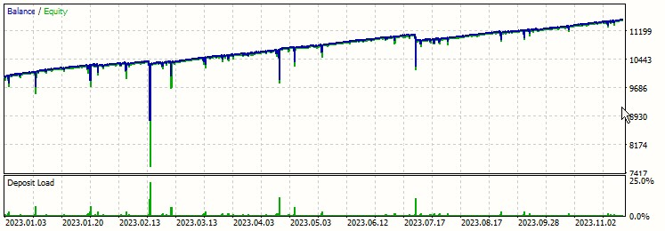
Just by looking at the graph, you might think that this is a profitable strategy but let's look at other data and discuss few points in the graph:
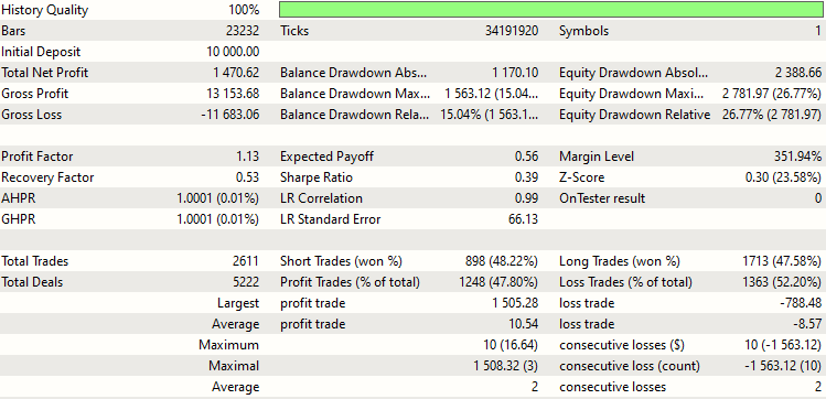
As you can see we had a net profit of $1470.62 where gross profit was $13,153.68 and gross loss was $11683.06.
Also, let's take a look at balance and equity drawdown:
| Balance Drawdown Absolute | $1170.10 |
| Balance Drawdown Maximal | $1563.12 (15.04%) |
| Balance Drawdown Relative | 15.04% ($1563.13) |
| Equity Drawdown Absolute | $2388.66 |
| Equity Drawdown Maximal | $2781.97 (26.77%) |
| Equity Drawdown Relative | 26.77% ($2781.97) |
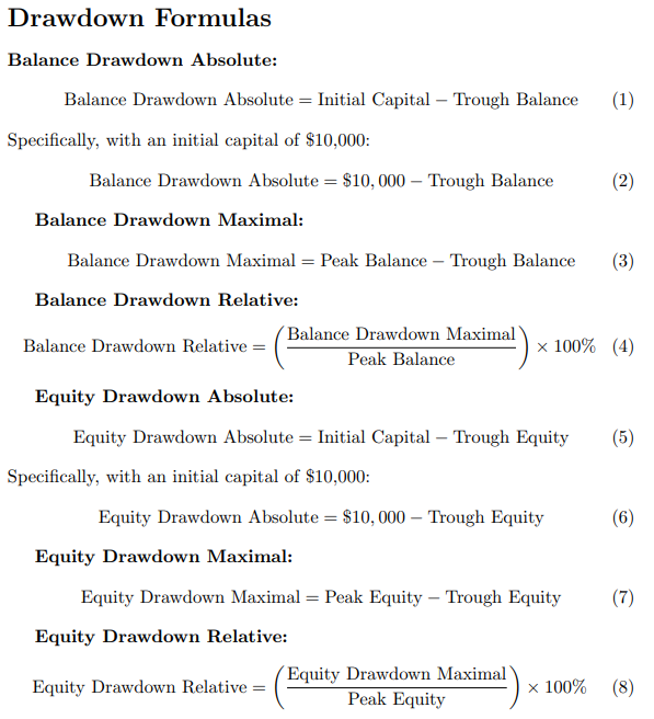
Let's understand these terms:
- Balance Drawdown Absolute: This is the difference between initial capital that is $10,000 in our case minus the minimum balance which is the lowest point of balance (trough balance).
- Balance Drawdown Maximal: This is the difference between highest point of balance (peak balance) minus the lowest point of balance (trough balance).
- Balance Drawdown Relative: This is the percentage of balance drawdown maximal out of highest point of balance (peak balance).
Equity definitions are symmetrical:
- Equity Drawdown Absolute: This is the difference between initial capital that is $10,000 in our case minus the minimum equity which is the lowest point of equity (trough equity).
- Equity Drawdown Maximal: This is the difference between highest point of equity (peak equity) minus the lowest point of equity (trough equity).
- Equity Drawdown Relative: This is the percentage of equity drawdown maximal out of highest point of equity (peak equity).
Below are the fomulas for all the 6 statistics:
Analysing the above data, balance drawdowns would be the least of our concerns as equity drawdowns covers that. In a sense we can say balance drawdowns are subsets of equity drawdowns. Also, Equity drawdowns are our biggest problem when following our strategy because we are doubling the lot size by 2 in each order that leads to an exponential growth of lot size which can be visualized by below table:
| Number of positions opened | Lot Size of next position (not opened yet) | Required Margin for the next position (EURUSD) |
|---|---|---|
| 0 | 0.01 | $2.16 |
| 1 | 0.02 | $4.32 |
| 2 | 0.04 | $8.64 |
| 3 | 0.08 | $17.28 |
| 4 | 0.16 | $34.56 |
| 5 | 0.32 | $69.12 |
| 6 | 0.64 | $138.24 |
| 7 | 1.28 | $276.48 |
| 8 | 2.56 | $552.96 |
| 9 | 5.12 | $1105.92 |
| 10 | 10.24 | $2211.84 |
| 11 | 20.48 | $4423.68 |
| 12 | 40.96 | $8847.36 |
| 13 | 80.92 | $17694.72 |
| 14 | 163.84 | $35389.44 |
In our exploration, we're currently utilizing EURUSD as our trading pair. It's important to note that the required margin for a 0.01 lot size stands at $2.16, although this figure is subject to change.
As we delve deeper, we observe a noteworthy trend: the required margin for subsequent positions increases exponentially. For instance, after the 12th order, we hit a financial bottleneck. The required margin soars to $17,694.44, a figure well beyond our reach considering our initial investment was $10,000. This scenario doesn't even take into account our stop-losses.
Let's break it down further. If we were to include stop-losses, set at 15 pips per trade, and having lost the first 12 trades, our cumulative lot size would be a staggering 81.91 (the sum of the series: 0.01+0.02+0.04+...+20.48+40.96). This translates to a total loss of $12,286.5, calculated using the EURUSD value of $1 per 10 pips for a 0.01 lot size. It's a simple calculation: (81.91/0.01) * 1.5 = $12,286.5. The loss not only exceeds our initial capital but also makes it impossible to sustain 12 positions in a cycle with a $10,000 investment in EURUSD.
Let's consider a slightly different scenario: Can we manage to sustain 11 total positions with our $10,000 in EURUSD?
Imagine we've reached 10 total positions. This implies we've already encountered stop losses on 9 positions and are about to lose the 10th. If we plan to open an 11th position, the total lot size for the 10 positions would be 10.23, leading to a loss of $1,534.5. This is calculated in the same manner as before, considering the EURUSD rate and lot size. The required margin for the next position would be $4,423.68. Summing up these amounts, we get $5,958.18, which is comfortably below our $10,000 threshold. Hence, it's feasible to survive 10 total positions and open an 11th.
However, the question arises: Is it possible to stretch to 12 total positions with the same $10,000?
For this, let's assume we've reached the brink of 11 positions. Here, we've already suffered losses on 10 positions and are on the verge of losing the 11th. The total lot size for these 11 positions is 20.47, resulting in a loss of $3,070.5. Adding the required margin for the 12th position, which is a hefty $8,847.36, our total expenditure rockets to $11,917.86, exceeding our initial investment. Therefore, it's clear that opening a 12th position with 11 already in play is financially untenable. We would have already lost $3,070.5, leaving us with just $6,929.5.
From the backtest statistics, we observe that the strategy is precariously close to collapse even with a $10,000 investment in a relatively stable currency like EURUSD. The maximum consecutive losses stand at 10, indicating we were just a few pips away from the disastrous 11th position. Should the 11th position also hit its stop loss, the strategy would unravel, leading to significant losses.
In our report, the absolute drawdown is marked at $2,388.66. Had we reached the 11th position's stop loss, our losses would have escalated to $3,070.5. This would have placed us $681.84 ($3,070.5 - $2,388.66) short of a total strategy failure.
However, there's a critical factor we've overlooked until now – the spread. This variable can significantly impact profits, as evidenced by two specific instances in our report, highlighted in the image below.
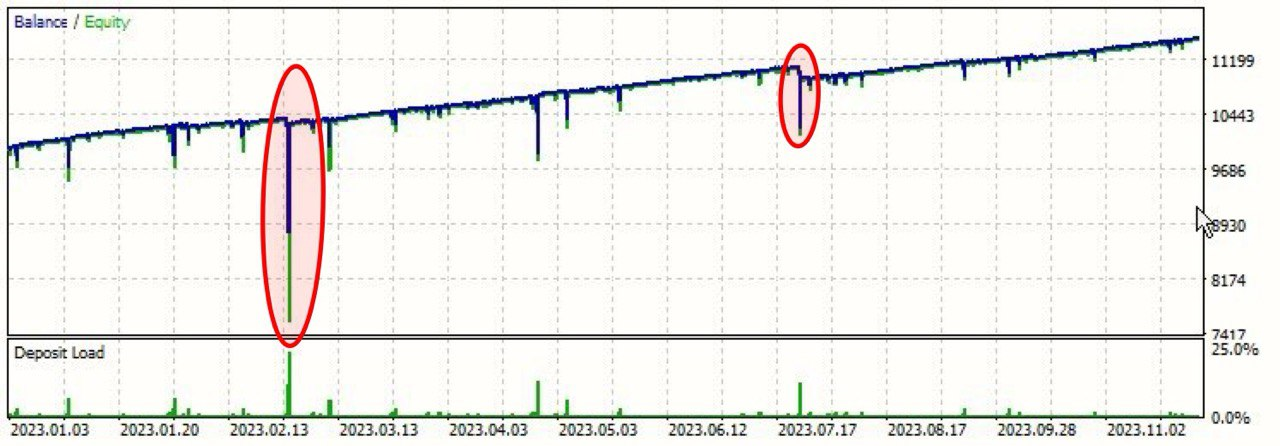
Notice the red circles in the image. In these cases, despite winning the trade (where winning equates to securing the highest lot in the last trade), we failed to realize any profit. This anomaly is attributed to the spread. Its variable nature further complicates our strategy, necessitating a more in-depth analysis in the next part of this series.
We must also consider the limitations of the classic hedge strategy. One significant drawback is the substantial holding capacity required to sustain numerous orders if the take profit level isn't reached early. This strategy can only assure profits if the lot size multiplier is 2 or greater (in case buyTP = sellTP = buySellDiff, ignoring the spread). If it's less than 2, there's a risk of incurring negative profits as the number of orders increases. We will explore these dynamics and how to optimize the classic hedge strategy for maximum returns in the upcoming part of our series.
Conclusion
So, we discussed quite a complex strategy in this first part of our series and also we automated it using Expert Advisor in MQL5. It can be a profitable strategy, although one must have a high holding capacity to place higher lot size positions which is not always feasible for an investor and also very risky as it might happen that he face a huge drawdown. To overcome these limitations we must optimise the strategy which will be done in next part of this series.
Till now we have been using arbitrary fixed values of lotSizeMultiplier, initialLotSize, buySellDiff, sellTP, buyTP but we can optimise this strategy and find optimal values of these input parameters that gives us maximum possible returns. Also we will find out whether it is beneficial to start initially with buy or sell position, that might also depend on different currencies and market conditions. So we will be covering a lot of useful things in next part of this series, so stay tuned for that.
Thank you for taking the time to read my articles. I hope you find them to be both informative and helpful in your endeavors. If you have any ideas or suggestions for what you'd like to see in my next piece, please don't hesitate to share.
Happy Coding! Happy Trading!
Warning: All rights to these materials are reserved by MetaQuotes Ltd. Copying or reprinting of these materials in whole or in part is prohibited.
This article was written by a user of the site and reflects their personal views. MetaQuotes Ltd is not responsible for the accuracy of the information presented, nor for any consequences resulting from the use of the solutions, strategies or recommendations described.

- Free trading apps
- Over 8,000 signals for copying
- Economic news for exploring financial markets
You agree to website policy and terms of use
I'll second that before this goes any further.
Hedging is not about counter orders at all. It is about related markets and derivatives. A EURUSD transaction can be hedged with EUR bonds, treasuries, their futures and options on them. All at once or individually. But not by EURUSD counter trade. A counter trade is a lock, it is a voluntary gift to a dealer/broker. Only if you are his relative and it is his birthday.
To check the strategy/principle for "whether it is not dumb or wishful thinking", you need to see how everything looks like in netting accounting and in multi-currency basket.
Ok, I accept my mistake but I only meant to connect with the readers. I have done a lot of freelance work and no one, absolutely no one ever called this Avalanche or Flip Trading System. Everyone there call this strategy as Hedging Strategy. So I assumed that hedging would better connect me with my readers.
So, yes technically I may be wrong, but I believe I have achieved my goal to connecting with the readers. Also since this terminology has been consistently used throughout the series, it would be challenging to revise it in all instances.
In addition, many readers have contacted me personally with their doubts, and judging from their questions the overall feedback I've received indicates that readers are familiar with and understand the strategy as described. Therefore, I believe it is more beneficial to maintain the current terminology to ensure consistency and understanding for all readers.
Anyway, thank you very much for letting me know my technical mistake.
Okay, I admit my mistake, but I just wanted to connect with readers. I've done a lot of freelancing and no one, absolutely no one has ever called this system Avalanche or Flip Trading System. Everyone calls this strategy a hedging strategy. So I assumed that hedging would better connect me with my readers.
So yes, technically I could be wrong, but I believe I achieved my goal of connecting with my readers. Also, since this terminology has been used consistently throughout the series, it would be difficult to revise it in all cases.
In addition, many readers have approached me personally with their concerns, and judging from their questions, the overall feedback I have received indicates that readers are familiar with and understand the strategy described. Therefore, I believe it is more beneficial to retain the current terminology to ensure consistency and understanding for all readers.
In any case, thank you very much for pointing out my technical error.
نعم إنه كذلك. ولكن هذا ليس سوى الجزء الأول، والفكرة الرئيسية هي متعددة العدد في هذا، والتي يتم تغطيتها في المزيد من المقالات وما يؤثر على التقدم.
thank u