
Data Science and Machine Learning (Part 16): A Refreshing Look at Decision Trees

Quick Recap
I wrote an article on decision trees in this article series that explained what decision trees are all about, and we built an algorithm to help us classify the weather data. However, the code and explanations provided in the article weren't concise enough; as I keep getting requests to provide a better approach to building decision trees, I believe writing a second article and providing better code for the decision tree might be better. Clarifying the decision trees will make it easier to understand the random forest algorithms that an article is coming out shortly.
What is a Decision Tree?
A Decision Tree is a flowchart-like tree structure where each internal Node represents a test on an attribute (or feature), each branch represents the outcome of the test, and each leaf Node represents a class label or a continuous value. The topmost Node in a decision tree is known as the "root," and the leaves are the outcomes or predictions.
What is a Node?
In a decision tree, a node is a fundamental component representing a decision point based on a particular feature or attribute. There are two main types of nodes in a decision tree: internal nodes and leaf nodes.
Internal Node- An internal node is a decision point in the tree where a test is performed on a specific feature. The test relies on a particular condition, such as whether a feature value is greater than a threshold or belongs to a particular category.
- Internal nodes have branches (edges) leading to child nodes. The outcome of the test determines which branch to follow.
- The internal Nodes, which are two left and right child nodes, are Nodes inside the central tree node.
- A leaf node marks a terminal point in the tree where it makes a final decision or prediction. It denotes the class label in a classification task or the predicted value in a regression task.
- Leaf nodes have no outgoing branches; they are the endpoints of the decision process.
- We will code this as a double variable.
class Node
{
  public:
    // for decision node

    uint feature_index;
    double threshold;
    double info_gain;

    // for leaf node

    double leaf_value;

    Node *left_child;  //left child Node
    Node *right_child; //right child Node

    Node() : left_child(NULL), right_child(NULL) {} // default constructor

    Node(uint feature_index_, double threshold_=NULL, Node *left_=NULL, Node *right_=NULL, double info_gain_=NULL, double value_=NULL)
        : left_child(left_), right_child(right_)
    {
        this.feature_index = feature_index_;
        this.threshold = threshold_;
        this.info_gain = info_gain_;
        this.value = value_;
    }

   void Print()
    {
      printf("feature_index: %d \nthreshold: %f \ninfo_gain: %f \nleaf_value: %f",feature_index,threshold, info_gain, value);
    }
};
Unlike some ML algorithms we have coded from scratch in this series, the decision tree can be tricky to code and confusing at times, as it requires recursive classes and functions to implement well, something that can be hard to code in a language other than Python, according to my experience.
Components of a Node:
A node in a decision tree typically contains the following information:
01. Test condition
Internal nodes have a test condition based on a specific feature and a threshold or category. This condition determines how the data is split into child nodes.
Node *build_tree(matrix &data, uint curr_depth=0);
02. Feature and Threshold
Indicates which feature is being tested at the node and the threshold or category used for the split.
uint feature_index;
double threshold;
03. Class Label or Value
A leaf node stores the predicted class label (for classification) or value (for regression)
double leaf_value; 04. Child Nodes
Internal nodes have child nodes corresponding to the different outcomes of the test condition. Each child node represents a subset of the data that satisfies the condition.
Node *left_child;  //left child Node
Node *right_child; //right child Node
Example:
Consider a simple decision tree for classifying whether a fruit is an apple or an orange based on its color;
[Node]
feature: color
Test condition: is the color Red?
If True, go to the left child; if False, go to the right child
[Leaf Node - Apple]
-Class label: Apple
[Leaf Node - Orange]
-Class label: Orange
Types of Decision Trees:
CART (Classification and Regression Trees): Used for both classification and regression tasks. Splits the data based on the Gini impurity for classification and mean squared error for regression.
ID3 (Iterative Dichotomiser 3): Primarily used for classification tasks. Employs the concept of entropy and information gain to make decisions.
C4.5: An improved version of ID3, C4.5, is used for classification. It employs a gain ratio to address bias towards attributes with more levels.
Since we will be looking to use the decision tree for classification purposes, we will be looking to build the ID3 algorithm characterized by Information gain, Impurity calculation and categorical features:
ID3 (Iterative Dichotomiser 3)
ID3 uses Information Gain to decide which feature to split on at each internal node. Information gain measures the reduction in entropy or uncertainty after a dataset is split.double CDecisionTree::information_gain(vector &parent, vector &left_child, vector &right_child) { double weight_left = left_child.Size() / (double)parent.Size(), weight_right = right_child.Size() / (double)parent.Size(); double gain =0; switch(m_mode) { case MODE_GINI: gain = gini_index(parent) - ( (weight_left*gini_index(left_child)) + (weight_right*gini_index(right_child)) ); break; case MODE_ENTROPY: gain = entropy(parent) - ( (weight_left*entropy(left_child)) + (weight_right*entropy(right_child)) ); break; } return gain; }
Entropy is a measure of uncertainty or disorder in a dataset. In ID3, the algorithm seeks to reduce entropy by choosing feature splits that result in subsets with more homogenous class labels.
double CDecisionTree::entropy(vector &y)
 {
   vector class_labels = matrix_utils.Unique_count(y);

   vector p_cls = class_labels / double(y.Size());

   vector entropy = (-1 * p_cls) * log2(p_cls);

  return entropy.Sum();
 }
To give more flexibility, one can choose between entropy and the Gini index, which is also a function often used in decision trees that does the same work as the entropy function. They both evaluate the impurity or disorder in the dataset.
double CDecisionTree::gini_index(vector &y)
 {
   vector unique = matrix_utils.Unique_count(y);

   vector probabilities = unique / (double)y.Size();

   return 1.0 - MathPow(probabilities, 2).Sum();
 }
Given by the formulas in the image below:
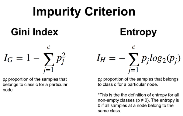
ID3 is particularly suitable for Categorical Features, and the selection of features and thresholds is based on the entropy reduction for categorical splits. We'll see this in action on the decision tree algorithm below.
Decision Tree Algorithm
01. Splitting Criteria
For classification, standard splitting criteria are Gini impurity and entropy, while mean squared error is often used for regression. Let's delve into the decision tree algorithm's splitting functions, which begin with the structure to retain information for the data undergoing a split.
//A struct containing splitted data information
struct split_info
  {
   uint feature_index;
   double threshold;
   matrix dataset_left,
          dataset_right;
   double info_gain;
  };
Using the threshold, we will split the features with values less than the threshold to the matrix dataset_left while keeping the rest to the matrix dataset_right. Lastly, the split_info structure instance is returned.
split_info CDecisionTree::split_data(const matrix &data, uint feature_index, double threshold=0.5)
 {
   int left_size=0, right_size =0;
   vector row = {};

   split_info split;

   ulong cols = data.Cols();

   split.dataset_left.Resize(0, cols);
   split.dataset_right.Resize(0, cols);

    for (ulong i=0; i<data.Rows(); i++)
     {
       row = data.Row(i);

       if (row[feature_index] <= threshold)
        {
          left_size++;
          split.dataset_left.Resize(left_size, cols);
          split.dataset_left.Row(row, left_size-1);
        }
       else
        {
         right_size++;
         split.dataset_right.Resize(right_size, cols);
         split.dataset_right.Row(row, right_size-1);
        }
     }
   return split;
 }
Out of many splits, the algorithm needs to figure out the best splits, the one with the maximum information gain.
split_info CDecisionTree::get_best_split(matrix &data, uint num_features)
  {

   double max_info_gain = -DBL_MAX;
   vector feature_values = {};
   vector left_v={}, right_v={}, y_v={};

//---

   split_info best_split;
   split_info split;

   for (uint i=0; i<num_features; i++)
     {
       feature_values = data.Col(i);
       vector possible_thresholds = matrix_utils.Unique(feature_values); //Find unique values in the feature, representing possible thresholds for splitting.

         for (uint j=0; j<possible_thresholds.Size(); j++)
            {
              split = this.split_data(data, i, possible_thresholds[j]);

              if (split.dataset_left.Rows()>0 && split.dataset_right.Rows() > 0)
                {
                  y_v = data.Col(data.Cols()-1);
                  right_v = split.dataset_right.Col(split.dataset_right.Cols()-1);
                  left_v = split.dataset_left.Col(split.dataset_left.Cols()-1);

                  double curr_info_gain = this.information_gain(y_v, left_v, right_v);

                  if (curr_info_gain > max_info_gain) // Check if the current information gain is greater than the maximum observed so far.
                    {
                      #ifdef DEBUG_MODE
                        printf("split left: [%dx%d] split right: [%dx%d] curr_info_gain: %f max_info_gain: %f",split.dataset_left.Rows(),split.dataset_left.Cols(),split.dataset_right.Rows(),split.dataset_right.Cols(),curr_info_gain,max_info_gain);
                      #endif

                      best_split.feature_index = i;
                      best_split.threshold = possible_thresholds[j];
                      best_split.dataset_left = split.dataset_left;
                      best_split.dataset_right = split.dataset_right;
                      best_split.info_gain = curr_info_gain;

                      max_info_gain = curr_info_gain;
                    }
                }
            }
     }

    return best_split;
  }
This function searches overall features and possible thresholds to find the best split that maximizes information gain. The result is a split_info structure containing information about the feature, threshold, and subsets associated with the best split.
02. Building the Tree
Decision Trees are constructed by recursively splitting the dataset based on features until a stopping condition is met (e.g., reaching a certain depth or minimum samples).
Node *CDecisionTree::build_tree(matrix &data, uint curr_depth=0)
 {
    matrix X;
    vector Y;

    matrix_utils.XandYSplitMatrices(data,X,Y); //Split the input matrix into feature matrix X and target vector Y.

    ulong samples = X.Rows(), features = X.Cols(); //Get the number of samples and features in the dataset.

    Node *node= NULL; // Initialize node pointer

    if (samples >= m_min_samples_split && curr_depth<=m_max_depth)
      {
         split_info best_split = this.get_best_split(data, (uint)features);

         #ifdef DEBUG_MODE
          Print("best_split left: [",best_split.dataset_left.Rows(),"x",best_split.dataset_left.Cols(),"]\nbest_split right: [",best_split.dataset_right.Rows(),"x",best_split.dataset_right.Cols(),"]\nfeature_index: ",best_split.feature_index,"\nInfo gain: ",best_split.info_gain,"\nThreshold: ",best_split.threshold);
         #endif

         if (best_split.info_gain > 0)
           {
             Node *left_child = this.build_tree(best_split.dataset_left, curr_depth+1);
             Node *right_child = this.build_tree(best_split.dataset_right, curr_depth+1);

             node = new Node(best_split.feature_index,best_split.threshold,left_child,right_child,best_split.info_gain);
             return node;
           }
      }

     node = new Node();
     node.leaf_value = this.calculate_leaf_value(Y);

     return node;
 }
if (best_split.info_gain > 0):
The above line of code checks if there is information gained.
Inside this block:
Node *left_child = this.build_tree(best_split.dataset_left, curr_depth+1);
Recursively build the left child node.
Node *right_child = this.build_tree(best_split.dataset_right, curr_depth+1);
Recursively build the right child node.
node = new Node(best_split.feature_index, best_split.threshold, left_child, right_child, best_split.info_gain);
Create a decision node with the information from the best split.
node = new Node(); If no further split is needed, create a new leaf node.
node.value = this.calculate_leaf_value(Y); Set the value of the leaf node using the calculate_leaf_value function.
return node; Return the node representing the current split or leaf.
To make the functions convenient and user-friendly, the build_tree function can be kept inside the fit function, which is commonly used in Python machine-learning modules.
void CDecisionTree::fit(matrix &x, vector &y)
 {
   matrix data = matrix_utils.concatenate(x, y, 1);

   this.root = this.build_tree(data);
 }
Making Predictions on Training and Testing of the Model
vector CDecisionTree::predict(matrix &x)
 {
    vector ret(x.Rows());

    for (ulong i=0; i<x.Rows(); i++)
       ret[i] = this.predict(x.Row(i));

   return ret;
 }
Making Predictions in Real-Time
double CDecisionTree::predict(vector &x)
 {
   return this.make_predictions(x, this.root);
 }
The make_predictions function is where all the dirty work gets done:
double CDecisionTree::make_predictions(vector &x, const Node &tree)
 {
    if (tree.leaf_value != NULL) // This is a leaf leaf_value
      return tree.leaf_value;

    double feature_value = x[tree.feature_index];
    double pred = 0;

    #ifdef DEBUG_MODE
      printf("Tree.threshold %f tree.feature_index %d leaf_value %f",tree.threshold,tree.feature_index,tree.leaf_value);
    #endif

    if (feature_value <= tree.threshold)
      {
       pred = this.make_predictions(x, tree.left_child);
      }
    else
     {
       pred = this.make_predictions(x, tree.right_child);
     }

   return pred;
 }
More details on this function:
if (feature_value <= tree.threshold): Inside this block:
Recursively call make_predictions for the left child node.
pred = this.make_predictions(x, *tree.left_child); Else, If the feature value is greater than the threshold:
Recursively call the make_predictions function for the right child node.
pred = this.make_predictions(x, *tree.right_child); return pred; Return the prediction.
Leaf Value Calculations
The function below calculates the leaf value:
double CDecisionTree::calculate_leaf_value(vector &Y)
 {
   vector uniques = matrix_utils.Unique_count(Y);
   vector classes = matrix_utils.Unique(Y);

   return classes[uniques.ArgMax()];
 }
This function returns the element from Y with the highest count, effectively finding the most common element in the list.
Wrapping it all up in a CDecisionTree class
enum mode {MODE_ENTROPY, MODE_GINI};

class CDecisionTree
  {
CMatrixutils   matrix_utils;

protected:

   Node *build_tree(matrix &data, uint curr_depth=0);
   double  calculate_leaf_value(vector &Y);

//---

   uint m_max_depth;
   uint m_min_samples_split;

   mode m_mode;

   double  gini_index(vector &y);
   double  entropy(vector &y);
   double  information_gain(vector &parent, vector &left_child, vector &right_child);


   split_info  get_best_split(matrix &data, uint num_features);
   split_info  split_data(const matrix &data, uint feature_index, double threshold=0.5);

   double make_predictions(vector &x, const Node &tree);
   void delete_tree(Node* node);

public:
                     Node *root;

                     CDecisionTree(uint min_samples_split=2, uint max_depth=2, mode mode_=MODE_GINI);
                    ~CDecisionTree(void);

                     void fit(matrix &x, vector &y);
                     void print_tree(Node *tree, string indent=" ",string padl="");
                     double predict(vector &x);
                     vector predict(matrix &x);
  };
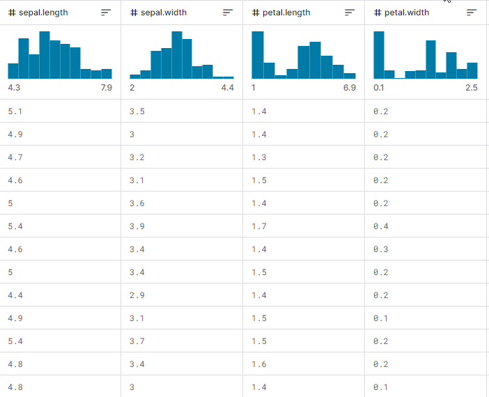
Having shown that, let us observe how everything works in action, how to build the tree, and how to use it to make predictions on training and testing, not to mention during real-time trading. We will use the most popular iris-CSV dataset to test if it does work.
Suppose we will be training the decision tree model on every EA initialization, starting by loading the training data from a CSV file:
int OnInit()
  {
  matrix dataset = matrix_utils.ReadCsv("iris.csv"); //loading iris-data

  decision_tree = new CDecisionTree(3,3, MODE_GINI); //Initializing the decision tree

  matrix x; vector y;
  matrix_utils.XandYSplitMatrices(dataset,x,y); //split the data into x and y matrix and vector respectively


  decision_tree.fit(x, y);  //Building the tree
  decision_tree.print_tree(decision_tree.root); //Printing the tree

  vector preds = decision_tree.predict(x); //making the predictions on a training data

  Print("Train Acc = ",metrics.confusion_matrix(y, preds)); //Measuring the accuracy

   return(INIT_SUCCEEDED);
  }
This is the appearance of the dataset matrix when printed. The last column has been Encoded. One(1) stands for Setosa, two(2) stands for Versicolor and three(3) stands for Virginica
Print("iris-csv\n",dataset);
MS      0       08:54:40.958    DecisionTree Test (EURUSD,H1)   iris-csv
PH      0       08:54:40.958    DecisionTree Test (EURUSD,H1)   [[5.1,3.5,1.4,0.2,1]
CO      0       08:54:40.958    DecisionTree Test (EURUSD,H1)    [4.9,3,1.4,0.2,1]
...
...

NS      0       08:54:40.959    DecisionTree Test (EURUSD,H1)    [5.6,2.7,4.2,1.3,2]
JK      0       08:54:40.959    DecisionTree Test (EURUSD,H1)    [5.7,3,4.2,1.2,2]
...
...

NQ      0       08:54:40.959    DecisionTree Test (EURUSD,H1)    [6.2,3.4,5.4,2.3,3]
PD      0       08:54:40.959    DecisionTree Test (EURUSD,H1)    [5.9,3,5.1,1.8,3]]
Printing the Tree
If you look at the code, you may have noticed the function print_tree, which takes the tree root as one of its arguments. This function attempts to print the overall tree appearance; a closer look below.
void CDecisionTree::print_tree(Node *tree, string indent=" ",string padl="")
  {
     if (tree.leaf_value != NULL)
        Print((padl+indent+": "),tree.leaf_value);
     else //if we havent' reached the leaf node keep printing child trees
       {
         padl += " ";

         Print((padl+indent)+": X_",tree.feature_index, "<=", tree.threshold, "?", tree.info_gain);

         print_tree(tree.left_child, "left","--->"+padl);

         print_tree(tree.right_child, "right","--->"+padl);
       }
  }
More details on this function:
Node Structure:
The function assumes that a Node class represents the decision tree. Each Node can be either a decision node or a leaf node. Decision nodes have a feature_index, a threshold, and an info_gain indicating the feature, threshold, information gain, and leaf_value.
Print Decision Node:
If the current Node is not a leaf node (i.e., tree.leaf_value is NULL), it prints information about the decision node. It prints the condition for the split, such as "X_2 <= 1.9 ? 0.33" and the indentation level.
Print Leaf Node:
If the current Node is a leaf node (i.e., tree.leaf_value is not NULL), it prints the leaf value along with the indentation level. For example, "left: 0.33".
Recursion:
The function then recursively calls itself for the left and right children of the current Node. The padl argument adds indentation to the printed output, making the tree structure more readable.
The output of the print_tree for the decision tree built inside the OnInit function is:
CR      0       09:26:39.990    DecisionTree Test (EURUSD,H1)     : X_2<=1.9?0.3333333333333334
HO      0       09:26:39.990    DecisionTree Test (EURUSD,H1)   ---> left: 1.0
RH      0       09:26:39.990    DecisionTree Test (EURUSD,H1)   --->  right: X_3<=1.7?0.38969404186795487
HP      0       09:26:39.990    DecisionTree Test (EURUSD,H1)   --->--->   left: X_2<=4.9?0.08239026063100136
KO      0       09:26:39.990    DecisionTree Test (EURUSD,H1)   --->--->--->    left: X_3<=1.6?0.04079861111111116
DH      0       09:26:39.990    DecisionTree Test (EURUSD,H1)   --->--->--->--->    left: 2.0
HM      0       09:26:39.990    DecisionTree Test (EURUSD,H1)   --->--->--->--->    right: 3.0
HS      0       09:26:39.990    DecisionTree Test (EURUSD,H1)   --->--->--->    right: X_3<=1.5?0.2222222222222222
IH      0       09:26:39.990    DecisionTree Test (EURUSD,H1)   --->--->--->--->    left: 3.0
QM      0       09:26:39.990    DecisionTree Test (EURUSD,H1)   --->--->--->--->    right: 2.0
KP      0       09:26:39.990    DecisionTree Test (EURUSD,H1)   --->--->   right: X_2<=4.8?0.013547574039067499
PH      0       09:26:39.990    DecisionTree Test (EURUSD,H1)   --->--->--->    left: X_0<=5.9?0.4444444444444444
PE      0       09:26:39.990    DecisionTree Test (EURUSD,H1)   --->--->--->--->    left: 2.0
DP      0       09:26:39.990    DecisionTree Test (EURUSD,H1)   --->--->--->--->    right: 3.0
EE      0       09:26:39.990    DecisionTree Test (EURUSD,H1)   --->--->--->   right: 3.0
Impressive.
Below is the accuracy of our trained Model:
  vector preds = decision_tree.predict(x); //making the predictions on a training data

  Print("Train Acc = ",metrics.confusion_matrix(y, preds)); //Measuring the accuracy
Outputs:
PM      0       09:26:39.990    DecisionTree Test (EURUSD,H1)   Confusion Matrix
CE      0       09:26:39.990    DecisionTree Test (EURUSD,H1)   [[50,0,0]
HR      0       09:26:39.990    DecisionTree Test (EURUSD,H1)    [0,50,0]
ND      0       09:26:39.990    DecisionTree Test (EURUSD,H1)    [0,1,49]]
GS      0       09:26:39.990    DecisionTree Test (EURUSD,H1)
KF      0       09:26:39.990    DecisionTree Test (EURUSD,H1)   Classification Report
IR      0       09:26:39.990    DecisionTree Test (EURUSD,H1)
MD      0       09:26:39.990    DecisionTree Test (EURUSD,H1)   _    Precision  Recall  Specificity  F1 score  Support
EQ      0       09:26:39.990    DecisionTree Test (EURUSD,H1)   1.0    50.00     50.00     100.00       50.00     50.0
HR      0       09:26:39.990    DecisionTree Test (EURUSD,H1)   2.0    51.00     50.00     100.00       50.50     50.0
PO      0       09:26:39.990    DecisionTree Test (EURUSD,H1)   3.0    49.00     50.00     100.00       49.49     50.0
EH      0       09:26:39.990    DecisionTree Test (EURUSD,H1)
PR      0       09:26:39.990    DecisionTree Test (EURUSD,H1)   Accuracy                                   0.99
HQ      0       09:26:39.990    DecisionTree Test (EURUSD,H1)   Average   50.00    50.00    100.00      50.00    150.0
DJ      0       09:26:39.990    DecisionTree Test (EURUSD,H1)   W Avg     50.00    50.00    100.00      50.00    150.0
LG      0       09:26:39.990    DecisionTree Test (EURUSD,H1)   Train Acc = 0.993
We achieved a 99.3% accuracy, indicating the successful implementation of our decision tree. This accuracy aligns with what you would expect from Scikit-Learn models when dealing with a simple dataset problem.
Let's proceed to train further and test the Model on out-of-sample data.
  matrix train_x, test_x;
  vector train_y, test_y;

  matrix_utils.TrainTestSplitMatrices(dataset, train_x, train_y, test_x, test_y, 0.8, 42); //split the data into training and testing samples


  decision_tree.fit(train_x, train_y);  //Building the tree
  decision_tree.print_tree(decision_tree.root); //Printing the tree

  vector preds = decision_tree.predict(train_x); //making the predictions on a training data

  Print("Train Acc = ",metrics.confusion_matrix(train_y, preds)); //Measuring the accuracy

//---

  preds = decision_tree.predict(test_x); //making the predictions on a test data

  Print("Test Acc = ",metrics.confusion_matrix(test_y, preds)); //Measuring the accuracy
Outputs:
QD      0       14:56:03.860    DecisionTree Test (EURUSD,H1)     : X_2<=1.7?0.34125
LL      0       14:56:03.860    DecisionTree Test (EURUSD,H1)   ---> left: 1.0
QK      0       14:56:03.860    DecisionTree Test (EURUSD,H1)   --->  right: X_3<=1.6?0.42857142857142855
GS      0       14:56:03.860    DecisionTree Test (EURUSD,H1)   --->--->   left: X_2<=4.9?0.09693877551020412
IL      0       14:56:03.860    DecisionTree Test (EURUSD,H1)   --->--->--->   left: 2.0
MD      0       14:56:03.860    DecisionTree Test (EURUSD,H1)   --->--->--->    right: X_3<=1.5?0.375
IS      0       14:56:03.860    DecisionTree Test (EURUSD,H1)   --->--->--->--->    left: 3.0
QR      0       14:56:03.860    DecisionTree Test (EURUSD,H1)   --->--->--->--->    right: 2.0
RH      0       14:56:03.860    DecisionTree Test (EURUSD,H1)   --->--->  right: 3.0
HP      0       14:56:03.860    DecisionTree Test (EURUSD,H1)   Confusion Matrix
FG      0       14:56:03.860    DecisionTree Test (EURUSD,H1)   [[42,0,0]
EO      0       14:56:03.860    DecisionTree Test (EURUSD,H1)    [0,39,0]
HK      0       14:56:03.860    DecisionTree Test (EURUSD,H1)    [0,0,39]]
OL      0       14:56:03.860    DecisionTree Test (EURUSD,H1)
KE      0       14:56:03.860    DecisionTree Test (EURUSD,H1)   Classification Report
QO      0       14:56:03.860    DecisionTree Test (EURUSD,H1)
MQ      0       14:56:03.860    DecisionTree Test (EURUSD,H1)   _    Precision  Recall  Specificity  F1 score  Support
OQ      0       14:56:03.860    DecisionTree Test (EURUSD,H1)   1.0    42.00     42.00     78.00       42.00     42.0
ML      0       14:56:03.860    DecisionTree Test (EURUSD,H1)   3.0    39.00     39.00     81.00       39.00     39.0
HK      0       14:56:03.860    DecisionTree Test (EURUSD,H1)   2.0    39.00     39.00     81.00       39.00     39.0
OE      0       14:56:03.860    DecisionTree Test (EURUSD,H1)
EO      0       14:56:03.860    DecisionTree Test (EURUSD,H1)   Accuracy                                   1.00
CG      0       14:56:03.860    DecisionTree Test (EURUSD,H1)   Average   40.00    40.00    80.00      40.00    120.0
LF      0       14:56:03.860    DecisionTree Test (EURUSD,H1)   W Avg     40.05    40.05    79.95      40.05    120.0
PR      0       14:56:03.860    DecisionTree Test (EURUSD,H1)   Train Acc = 1.0
CD      0       14:56:03.861    DecisionTree Test (EURUSD,H1)   Confusion Matrix
FO      0       14:56:03.861    DecisionTree Test (EURUSD,H1)   [[9,2,0]
RK      0       14:56:03.861    DecisionTree Test (EURUSD,H1)    [1,10,0]
CL      0       14:56:03.861    DecisionTree Test (EURUSD,H1)    [2,0,6]]
HK      0       14:56:03.861    DecisionTree Test (EURUSD,H1)
DQ      0       14:56:03.861    DecisionTree Test (EURUSD,H1)   Classification Report
JJ      0       14:56:03.861    DecisionTree Test (EURUSD,H1)
FM      0       14:56:03.861    DecisionTree Test (EURUSD,H1)   _    Precision  Recall  Specificity  F1 score  Support
QM      0       14:56:03.861    DecisionTree Test (EURUSD,H1)   2.0    12.00     11.00     19.00       11.48     11.0
PH      0       14:56:03.861    DecisionTree Test (EURUSD,H1)   3.0    12.00     11.00     19.00       11.48     11.0
KD      0       14:56:03.861    DecisionTree Test (EURUSD,H1)   1.0    6.00     8.00     22.00       6.86     8.0
PP      0       14:56:03.861    DecisionTree Test (EURUSD,H1)
LJ      0       14:56:03.861    DecisionTree Test (EURUSD,H1)   Accuracy                                   0.83
NJ      0       14:56:03.861    DecisionTree Test (EURUSD,H1)   Average   10.00    10.00    20.00      9.94    30.0
JR      0       14:56:03.861    DecisionTree Test (EURUSD,H1)   W Avg     10.40    10.20    19.80      10.25    30.0
HP      0       14:56:03.861    DecisionTree Test (EURUSD,H1)   Test Acc = 0.833
The model is 100% accurate on a training data while being 83% accurate on out-of-sample data.
Decision Tree AI in Trading
All this amounts to nothing if we don't explore the trading aspect using the decision tree models. To use this Model in trading, let us formulate a problem we want to solve.
The Problem To Solve:
We want to use the decision tree AI model to make predictions on the current bar to possibly tell us where the market is heading, either up or down.
As with any model, we want to give the Model a dataset to learn upon; let's say we decide to use the two indicators of oscillator types, The RSI indicator and the Stochastic oscillator; basically, We want the Model to understand the patterns between these two indicators and how it affects the price movement for the current bar.

Data structure:
Once collected for train-test purposes, the data gets stored in the structure below. The same applies to data used for making real-time predictions.
struct data{
   vector stoch_buff,
          signal_buff,
          rsi_buff,
          target;
} data_struct;
Collecting Data, Training and Testing the decision Tree
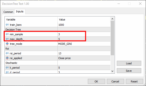
void TrainTree()
 {
  matrix dataset(train_bars, 4);
  vector v;

//--- Collecting indicator buffers

  data_struct.rsi_buff.CopyIndicatorBuffer(rsi_handle, 0, 1, train_bars);
  data_struct.stoch_buff.CopyIndicatorBuffer(stoch_handle, 0, 1, train_bars);
  data_struct.signal_buff.CopyIndicatorBuffer(stoch_handle, 1, 1, train_bars);

//--- Preparing the target variable

  MqlRates rates[];
  ArraySetAsSeries(rates, true);
  int size = CopyRates(Symbol(), PERIOD_CURRENT, 1,train_bars, rates);

  data_struct.target.Resize(size); //Resize the target vector

  for (int i=0; i<size; i++)
    {
      if (rates[i].close > rates[i].open)
        data_struct.target[i] = 1;
      else
        data_struct.target[i] = -1;
    }

  dataset.Col(data_struct.rsi_buff, 0);
  dataset.Col(data_struct.stoch_buff, 1);
  dataset.Col(data_struct.signal_buff, 2);
  dataset.Col(data_struct.target, 3);

  decision_tree = new CDecisionTree(min_sample,max_depth_, tree_mode); //Initializing the decision tree


  matrix train_x, test_x;
  vector train_y, test_y;

  matrix_utils.TrainTestSplitMatrices(dataset, train_x, train_y, test_x, test_y, 0.8, 42); //split the data into training and testing samples


  decision_tree.fit(train_x, train_y);  //Building the tree
  decision_tree.print_tree(decision_tree.root); //Printing the tree

  vector preds = decision_tree.predict(train_x); //making the predictions on a training data

  Print("Train Acc = ",metrics.confusion_matrix(train_y, preds)); //Measuring the accuracy

//---

  preds = decision_tree.predict(test_x); //making the predictions on a test data

  Print("Test Acc = ",metrics.confusion_matrix(test_y, preds)); //Measuring the accuracy
 }
Min-sample was set to 3 while the max-depth was set to 5.
Outputs:
KR      0       16:26:53.028    DecisionTree Test (EURUSD,H1)     : X_0<=65.88930872549261?0.0058610536710859695
CN      0       16:26:53.028    DecisionTree Test (EURUSD,H1)   --->  left: X_0<=29.19882857713344?0.003187469522387243
FK      0       16:26:53.028    DecisionTree Test (EURUSD,H1)   --->--->   left: X_1<=26.851851851853503?0.030198175526895188
RI      0       16:26:53.028    DecisionTree Test (EURUSD,H1)   --->--->--->    left: X_2<=7.319205739522295?0.040050858232676456
KG      0       16:26:53.028    DecisionTree Test (EURUSD,H1)   --->--->--->--->     left: X_0<=23.08345903222593?0.04347468770545693
JF      0       16:26:53.028    DecisionTree Test (EURUSD,H1)   --->--->--->--->--->      left: X_0<=21.6795921184317?0.09375
PF      0       16:26:53.028    DecisionTree Test (EURUSD,H1)   --->--->--->--->--->--->      left: -1.0
ER      0       16:26:53.028    DecisionTree Test (EURUSD,H1)   --->--->--->--->--->--->      right: -1.0
QF      0       16:26:53.028    DecisionTree Test (EURUSD,H1)   --->--->--->--->--->      right: X_2<=3.223853479489069?0.09876543209876543
LH      0       16:26:53.028    DecisionTree Test (EURUSD,H1)   --->--->--->--->--->--->      left: -1.0
FJ      0       16:26:53.028    DecisionTree Test (EURUSD,H1)   --->--->--->--->--->--->      right: 1.0
MM      0       16:26:53.028    DecisionTree Test (EURUSD,H1)   --->--->--->--->    right: -1.0
MG      0       16:26:53.028    DecisionTree Test (EURUSD,H1)   --->--->--->   right: 1.0
HH      0       16:26:53.028    DecisionTree Test (EURUSD,H1)   --->--->   right: X_0<=65.4606831930956?0.0030639039663222234
JR      0       16:26:53.028    DecisionTree Test (EURUSD,H1)   --->--->--->    left: X_0<=31.628407983040333?0.00271101025966336
PS      0       16:26:53.028    DecisionTree Test (EURUSD,H1)   --->--->--->--->     left: X_0<=31.20436037455599?0.0944903581267218
DO      0       16:26:53.028    DecisionTree Test (EURUSD,H1)   --->--->--->--->--->      left: X_2<=14.629981942657205?0.11111111111111116
EO      0       16:26:53.028    DecisionTree Test (EURUSD,H1)   --->--->--->--->--->--->      left: 1.0
IG      0       16:26:53.028    DecisionTree Test (EURUSD,H1)   --->--->--->--->--->--->      right: -1.0
EI      0       16:26:53.028    DecisionTree Test (EURUSD,H1)   --->--->--->--->--->     right: 1.0
LO      0       16:26:53.028    DecisionTree Test (EURUSD,H1)   --->--->--->--->     right: X_0<=32.4469112469684?0.003164795835173595
RO      0       16:26:53.028    DecisionTree Test (EURUSD,H1)   --->--->--->--->--->      left: X_1<=76.9736842105244?0.21875
RO      0       16:26:53.028    DecisionTree Test (EURUSD,H1)   --->--->--->--->--->--->      left: -1.0
PG      0       16:26:53.028    DecisionTree Test (EURUSD,H1)   --->--->--->--->--->--->      right: 1.0
MO      0       16:26:53.028    DecisionTree Test (EURUSD,H1)   --->--->--->--->--->      right: X_0<=61.82001028403415?0.0024932856070305487
LQ      0       16:26:53.028    DecisionTree Test (EURUSD,H1)   --->--->--->--->--->--->      left: -1.0
EQ      0       16:26:53.029    DecisionTree Test (EURUSD,H1)   --->--->--->--->--->--->      right: 1.0
LE      0       16:26:53.029    DecisionTree Test (EURUSD,H1)   --->--->--->    right: X_2<=84.68660541575225?0.09375
ED      0       16:26:53.029    DecisionTree Test (EURUSD,H1)   --->--->--->--->    left: -1.0
LM      0       16:26:53.029    DecisionTree Test (EURUSD,H1)   --->--->--->--->    right: -1.0
NE      0       16:26:53.029    DecisionTree Test (EURUSD,H1)   --->  right: X_0<=85.28191275702572?0.024468404842877933
DK      0       16:26:53.029    DecisionTree Test (EURUSD,H1)   --->--->   left: X_1<=25.913621262458935?0.01603292204455742
LE      0       16:26:53.029    DecisionTree Test (EURUSD,H1)   --->--->--->    left: X_0<=72.18709160232456?0.2222222222222222
ED      0       16:26:53.029    DecisionTree Test (EURUSD,H1)   --->--->--->--->     left: X_1<=15.458937198072245?0.4444444444444444
QQ      0       16:26:53.029    DecisionTree Test (EURUSD,H1)   --->--->--->--->--->     left: 1.0
CS      0       16:26:53.029    DecisionTree Test (EURUSD,H1)   --->--->--->--->--->     right: -1.0
JE      0       16:26:53.029    DecisionTree Test (EURUSD,H1)   --->--->--->--->    right: -1.0
QM      0       16:26:53.029    DecisionTree Test (EURUSD,H1)   --->--->--->    right: X_0<=69.83504428897093?0.012164425148527835
HP      0       16:26:53.029    DecisionTree Test (EURUSD,H1)   --->--->--->--->     left: X_0<=68.39798826749553?0.07844460227272732
DL      0       16:26:53.029    DecisionTree Test (EURUSD,H1)   --->--->--->--->--->      left: X_1<=90.68322981366397?0.06611570247933873
DO      0       16:26:53.029    DecisionTree Test (EURUSD,H1)   --->--->--->--->--->--->      left: 1.0
OE      0       16:26:53.029    DecisionTree Test (EURUSD,H1)   --->--->--->--->--->--->      right: 1.0
LI      0       16:26:53.029    DecisionTree Test (EURUSD,H1)   --->--->--->--->--->      right: X_1<=88.05704099821516?0.11523809523809525
DE      0       16:26:53.029    DecisionTree Test (EURUSD,H1)   --->--->--->--->--->--->      left: 1.0
DM      0       16:26:53.029    DecisionTree Test (EURUSD,H1)   --->--->--->--->--->--->      right: -1.0
LG      0       16:26:53.029    DecisionTree Test (EURUSD,H1)   --->--->--->--->     right: X_0<=70.41747488780877?0.015360959832756427
OI      0       16:26:53.029    DecisionTree Test (EURUSD,H1)   --->--->--->--->--->     left: 1.0
PI      0       16:26:53.029    DecisionTree Test (EURUSD,H1)   --->--->--->--->--->      right: X_0<=70.56490391752676?0.02275277028755862
CF      0       16:26:53.029    DecisionTree Test (EURUSD,H1)   --->--->--->--->--->--->      left: -1.0
MO      0       16:26:53.029    DecisionTree Test (EURUSD,H1)   --->--->--->--->--->--->      right: 1.0
EG      0       16:26:53.029    DecisionTree Test (EURUSD,H1)   --->--->   right: X_1<=97.0643939393936?0.10888888888888892
CJ      0       16:26:53.029    DecisionTree Test (EURUSD,H1)   --->--->--->   left: 1.0
GN      0       16:26:53.029    DecisionTree Test (EURUSD,H1)   --->--->--->    right: X_0<=90.20261550045987?0.07901234567901233
CP      0       16:26:53.029    DecisionTree Test (EURUSD,H1)   --->--->--->--->     left: X_0<=85.94461490761033?0.21333333333333332
HN      0       16:26:53.029    DecisionTree Test (EURUSD,H1)   --->--->--->--->--->     left: -1.0
GE      0       16:26:53.029    DecisionTree Test (EURUSD,H1)   --->--->--->--->--->      right: X_1<=99.66856060606052?0.4444444444444444
GK      0       16:26:53.029    DecisionTree Test (EURUSD,H1)   --->--->--->--->--->--->      left: -1.0
IK      0       16:26:53.029    DecisionTree Test (EURUSD,H1)   --->--->--->--->--->--->      right: 1.0
JM      0       16:26:53.029    DecisionTree Test (EURUSD,H1)   --->--->--->--->    right: -1.0
KE      0       16:26:53.029    DecisionTree Test (EURUSD,H1)   Confusion Matrix
DO      0       16:26:53.029    DecisionTree Test (EURUSD,H1)   [[122,271]
QF      0       16:26:53.029    DecisionTree Test (EURUSD,H1)    [51,356]]
HS      0       16:26:53.029    DecisionTree Test (EURUSD,H1)
LF      0       16:26:53.029    DecisionTree Test (EURUSD,H1)   Classification Report
JR      0       16:26:53.029    DecisionTree Test (EURUSD,H1)
ND      0       16:26:53.029    DecisionTree Test (EURUSD,H1)   _    Precision  Recall  Specificity  F1 score  Support
GQ      0       16:26:53.029    DecisionTree Test (EURUSD,H1)   1.0    173.00     393.00     407.00       240.24     393.0
HQ      0       16:26:53.029    DecisionTree Test (EURUSD,H1)   -1.0    627.00     407.00     393.00       493.60     407.0
PM      0       16:26:53.029    DecisionTree Test (EURUSD,H1)
OG      0       16:26:53.029    DecisionTree Test (EURUSD,H1)   Accuracy                                   0.60
EO      0       16:26:53.029    DecisionTree Test (EURUSD,H1)   Average   400.00    400.00    400.00      366.92    800.0
GN      0       16:26:53.029    DecisionTree Test (EURUSD,H1)   W Avg     403.97    400.12    399.88      369.14    800.0
LM      0       16:26:53.029    DecisionTree Test (EURUSD,H1)   Train Acc = 0.598
GK      0       16:26:53.029    DecisionTree Test (EURUSD,H1)   Confusion Matrix
CQ      0       16:26:53.029    DecisionTree Test (EURUSD,H1)   [[75,13]
CK      0       16:26:53.029    DecisionTree Test (EURUSD,H1)    [86,26]]
NI      0       16:26:53.029    DecisionTree Test (EURUSD,H1)
RP      0       16:26:53.029    DecisionTree Test (EURUSD,H1)   Classification Report
HH      0       16:26:53.029    DecisionTree Test (EURUSD,H1)
LR      0       16:26:53.029    DecisionTree Test (EURUSD,H1)   _    Precision  Recall  Specificity  F1 score  Support
EM      0       16:26:53.029    DecisionTree Test (EURUSD,H1)   -1.0    161.00     88.00     112.00       113.80     88.0
NJ      0       16:26:53.029    DecisionTree Test (EURUSD,H1)   1.0    39.00     112.00     88.00       57.85     112.0
LJ      0       16:26:53.029    DecisionTree Test (EURUSD,H1)
EL      0       16:26:53.029    DecisionTree Test (EURUSD,H1)   Accuracy                                   0.51
RG      0       16:26:53.029    DecisionTree Test (EURUSD,H1)   Average   100.00    100.00    100.00      85.83    200.0
ID      0       16:26:53.029    DecisionTree Test (EURUSD,H1)   W Avg     92.68    101.44    98.56      82.47    200.0
JJ      0       16:26:53.029    DecisionTree Test (EURUSD,H1)   Test Acc = 0.505
The Model was correct 60% of the time during training while being 50.5% accurate during testing; not good. There might be many reasons, including the quality of the data we used to build the Model, or maybe there are bad predictors. The most common reason might be that we have not set the parameters for the Model well.
To fix this, you might need to tweak the parameters to determine what works best for your needs.
Now, let's code for a function to make real-time predictions.
int desisionTreeSignal()
 {
//--- Copy the current bar information only

   data_struct.rsi_buff.CopyIndicatorBuffer(rsi_handle, 0, 0, 1);
   data_struct.stoch_buff.CopyIndicatorBuffer(stoch_handle, 0, 0, 1);
   data_struct.signal_buff.CopyIndicatorBuffer(stoch_handle, 1, 0, 1);

   x_vars[0] = data_struct.rsi_buff[0];
   x_vars[1] = data_struct.stoch_buff[0];
   x_vars[2] = data_struct.signal_buff[0];

   return int(decision_tree.predict(x_vars));
 }
Now, let us make a simple trading logic:
If the decision tree predicts -1, meaning the candle will close down, we open a sell trade; if it predicts the class of 1, indicating the candle will close higher than where it opened, we want to place a buy trade.
void OnTick()
  {
//---
    if (!train_once)              // You want to train once during EA lifetime
      TrainTree();
    train_once = true;

    if (isnewBar(PERIOD_CURRENT)) // We want to trade on the bar opening
      {
        int signal = desisionTreeSignal();
        double min_lot = SymbolInfoDouble(Symbol(), SYMBOL_VOLUME_MIN);
        SymbolInfoTick(Symbol(), ticks);

         if (signal == -1)
           {
              if (!PosExists(MAGICNUMBER, POSITION_TYPE_SELL)) // If a sell trade doesnt exist
                m_trade.Sell(min_lot, Symbol(), ticks.bid, ticks.bid+stoploss*Point(), ticks.bid - takeprofit*Point());
           }
         else
           {
             if (!PosExists(MAGICNUMBER, POSITION_TYPE_BUY))  // If a buy trade doesnt exist
               m_trade.Buy(min_lot, Symbol(), ticks.ask, ticks.ask-stoploss*Point(), ticks.ask + takeprofit*Point());
           }
      }
  }
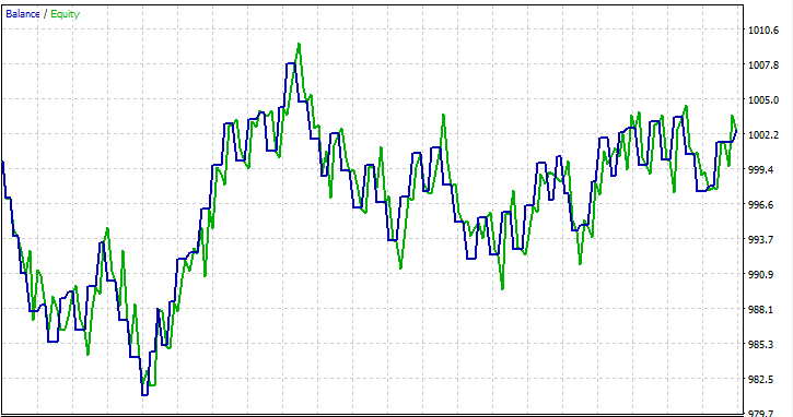
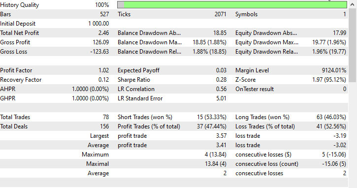
I ran a test on a single month 2023.01.01 - 2023.02.01 on Open Prices just to see if everything works out.
FAQs on Decision Trees in Trading:
| Question | Answer |
|---|---|
| Is normalization of input data important for decision trees? | No, normalization is generally not crucial for decision trees at all. Decision trees make splits based on feature thresholds, and the scale of features doesn't affect the tree structure. However, it's a good practice to check the impact of normalization on model performance. |
| How do decision trees handle categorical variables in trading data? | Decision trees can handle categorical variables naturally. They perform binary splits based on whether a condition is met, including conditions for categorical variables. The tree will determine the optimal split points for categorical features. |
| Can decision trees be used for time-series forecasting in trading? | While decision trees can be utilized for time-series forecasting in trading, they may not capture complex temporal patterns as effectively as models such as recurrent neural networks (RNNs). Ensemble methods like Random Forests could offer greater robustness |
| Do decision trees suffer from overfitting? | Decision trees, particularly deep ones, can be prone to overfitting by capturing noise in the training data. Techniques such as pruning and limiting tree depth can be employed to mitigate overfitting in trading applications |
| Are decision trees suitable for feature importance analysis in trading models? | Yes, decision trees provide a natural way to assess feature importance. Features that contribute more to the splitting decisions at the top of the tree are generally more critical. This analysis can offer insights into the factors driving trading decisions. |
| How sensitive are decision trees to outliers in trading data? | Decision trees can be sensitive to outliers, especially when the tree is deep. Outliers may lead to specific splits that capture noise. Preprocessing steps, such as outlier detection and removal, can be applied to mitigate this sensitivity. |
| Are there specific hyperparameters to tune for decision trees in trading models? | Yes, key hyperparameters to tune include
One can use Cross-validation to find optimal hyperparameter values for given datasets. |
| Can decision trees be part of an ensemble approach? | Yes, decision trees can be part of ensemble methods like Random Forests, which combine multiple trees to improve overall predictive performance. Ensemble methods are often robust and effective in trading applications. |
Advantages of Decision Trees:
Interpretability:
- Decision trees are easy to understand and interpret. The graphical representation of the tree structure allows for clear visualization of decision-making processes.
Handling Non-Linearity:
- Decision trees can capture non-linear relationships in data, making them suitable for problems where the decision boundaries are not linear.
Handling Mixed Data Types:
- Decision trees can take both numerical and categorical data without the need for extensive preprocessing.
Feature Importance:
- Decision trees provide a natural way to assess the importance of features, helping identify critical factors influencing the target variable.
No Assumptions about Data Distribution:
- Decision trees make no assumptions about data distribution, making them versatile and applicable to various datasets.
Robustness to Outliers:
- Decision trees are relatively robust to outliers since splits are based on relative comparisons and unaffected by absolute values.
Automatic Variable Selection:
- The tree-building process includes automatic variable selection, reducing the need for manual feature engineering.
Can Handle Missing Values:
- Decision trees can handle missing values in features without requiring imputation, as splits are made based on available data.
Disadvantages of Decision Trees:
Overfitting:
- Decision trees are prone to overfitting, especially when they are deep and capture noise in the training data. Techniques like pruning are used to address this issue.
Instability:
- Small changes in the data can lead to significant changes in the tree structure, making decision trees somewhat unstable.
Bias Toward Dominant Classes:
- In datasets with imbalanced classes, decision trees can be biased toward the dominant class, leading to suboptimal performance for minority classes.
Global Optimum vs. Local Optima:
- Decision trees focus on finding local optimum splits at each node, which may not necessarily lead to a globally optimal solution.
Limited Expressiveness:
- Decision trees might struggle to express complex relationships in data compared to more sophisticated models like neural networks.
Not Suitable for Continuous Output:
- While decision trees are adequate for classification tasks, they may not be as suitable for tasks requiring a continuous output.
Sensitive to Noisy Data:
- Decision trees can be sensitive to noisy data, and outliers may lead to specific splits that capture noise rather than meaningful patterns.
Biased Toward Dominant Features:
- Features with more levels or categories may appear more critical due to how splits are made, potentially introducing bias. One can address this through techniques like feature scaling.
That's it folks, Thanks for reading.
Track the development and contribute to the decision tree algorithm and many more AI models on my GitHub repo: https://github.com/MegaJoctan/MALE5/tree/master
Attachments:
| tree.mqh | The main include, file. Contains the decision tree code we mainly discussed above. |
| metrics.mqh | Contains functions and code to measure the performance of ML models. |
| matrix_utils.mqh | Contains additional functions for matrix manipulations. |
| preprocessing.mqh | The library for pre-processing raw input data to make it suitable for Machine learning models usage. |
| DecisionTree Test.mq5(EA) | The main file. An expert advisor for running the decision tree. |
Warning: All rights to these materials are reserved by MetaQuotes Ltd. Copying or reprinting of these materials in whole or in part is prohibited.
This article was written by a user of the site and reflects their personal views. MetaQuotes Ltd is not responsible for the accuracy of the information presented, nor for any consequences resulting from the use of the solutions, strategies or recommendations described.

 How to create a simple Multi-Currency Expert Advisor using MQL5 (Part 5): Bollinger Bands On Keltner Channel — Indicators Signal
- Free trading apps
- Over 8,000 signals for copying
- Economic news for exploring financial markets
You agree to website policy and terms of use