Neural networks made easy (Part 36): Relational Reinforcement Learning

Introduction
We continue to explore reinforcement learning methods. In the previous articles we already discussed several algorithms. But we always used convolutional models. The reason for this is simple. When designing and testing all the previously considered algorithms, we used various computer games. Therefore, we mainly fed into the models the images of levels of various computer games. Convolutional models can easily solve tasks related to image recognition and detection of objects on these images.
Images from computer games do not have noise or object distortions. This simplifies the recognition task. However, in reality there are no such "ideal" conditions. The data is full of various noises. Very often, the studied images are far from ideal expectations. They can be moved around the scene (convolutional networks can easily handle this), as well as subject to various distortions. They can also be stretched, compressed or presented at a different angle. This task is more difficult to handle for a usual convolutional model.
In some situations, not only the presence of two or more objects, but also their relative position is important for the successful solution of the problem. It is difficult to solve such problems using inly convolutional models. But they are well solved by relational models.
1. Relational Reinforcement Learning
The main advantage of relational models is the ability to build dependencies between objects. That enables the structuring of the source data. The relational model can be represented in the form of graphs, in which objects and events are represented as nodes, while relationships show dependencies between objects and events.

By using the graphs, we can visually build the structure of dependencies between objects. For example, if we want to describe a channel breakout pattern, we can draw up a graph with a channel formation at the top. The channel formation description can also be represented as a graph. Next, we will create two channel breakout nodes (upper and lower borders). Both nodes will have the same links to the previous channel formation node, but they are not connected to each other. To avoid entering a position in case of a false breakout, we can wait for the price to roll back to the channel border. These are two more nodes for the rollback to the upper and lower borders of the channel. They will have connections with the nodes of the corresponding channel border breakouts. But again, they will not have connections with each other.
The described structure fits into the graph and thus provides a clear structuring of data and of an event sequence. We considered something similar when constructing association rules. But this can hardly be related to the convolutional networks we used earlier.
Convolutional networks are used to identify objects in data. We can train the model to detect some movement reversal points or small trends. But in practice, the channel formation process can be extended in time with different intensity of trends within the channel. However, convolutional models may not cope well with such distortions. In addition, neither convolutional nor fully connected neural layers can separate two different patterns that consist of the same objects with a different sequence.
It should also be noted that convolutional neural networks can only detect objects, but they cannot build dependencies between them. Therefore, we need to find some other algorithm which can learn such dependencies. Now, let us get back to attention models. The attention models that make it possible to focus attention on individual objects, singling them out from the general data array.
The "generalized attention mechanism" was first proposed in September 2014 as an effort to improve the efficiency of machine translation models using recurrent models. The idea was to create an additional layer of attention, which would collect the hidden states of the encoder when processing the original dataset. This solved the problem of long-term memory. The analysis of dependencies between sequence elements helped to improve the quality of machine translation.
The mechanism operation algorithm included the following iterations:
1. Creating Encoder hidden states and accumulating them in the attention block.
2. Evaluating pairwise dependencies between the hidden states of each Encoder element and the last hidden state of the Decoder.
3. Combining the resulting scores into a single vector and normalizing them using the Softmax function.
4. Computing the context vector by multiplying all the hidden states of the Encoder by their corresponding alignment scores.
5. Decoding the context vector and combining the resulting value with the previous state of the Decoder.
All iterations are repeated until the end-of-sentence signal is received.
The figure below shows the visualization of this solution:

However, training recurrent models is a rather time-consuming process. So, in June 2017, another variation was proposed in article "Attention Is All You Need". This was a new architecture of the Transformer neural network, which did not use recurrent blocks, but used a new Self-Attention algorithm. Unlike the previously described algorithm, Self-Attention analyzes pairwise dependencies within one sequence. In previous articles, we have already created 3 types of neural layers using the Self Attention algorithm. We will use one of them in this article. But before proceeding with the implementation of the Expert Advisor, let us consider how the Self Attention algorithm can learn the graph structure.

At the input of the Self Attention algorithm, we expect a tensor of the source data, in which each element of the sequence is described by a certain number of features. The number of such features is predetermined, and it is fixed for all elements of the sequence. Thus, the initial data tensor is presented as a table. Each row of this table is a description of one element of the sequence. Each column corresponds to a single feature.
The features used can have completely different distributions. The distribution characteristics of one feature can be very different from those of another feature. The impact of absolute values of features and their changes on the final result can also be absolutely opposite. To bring the data into a comparable form, similarly to the hidden state of the recurrent layer, we use a weight matrix. Multiplying each row of the initial data tensor by the weight matrix transforms the description of the sequence element into a certain d-dimensional internal embedding space. The selection of parameters for the specified matrix in the learning process allows selection of the values for which the elements of the sequence will be maximally separable and will be grouped by similarity. Note that the Self Attention algorithm allows the creation and training of three such matrices. The matrices allow us to form three different source data embeddings: Query, Key and Value. The Query and Key vector dimensions are set during model creation. The Value vector dimension corresponds to the number of features in the source data (to the size of one element description vector).
Each of the generated embeddings has its own functional purpose. Query and Key are used to define interdependencies between sequence elements. Value defines which information from each element should be passed on.
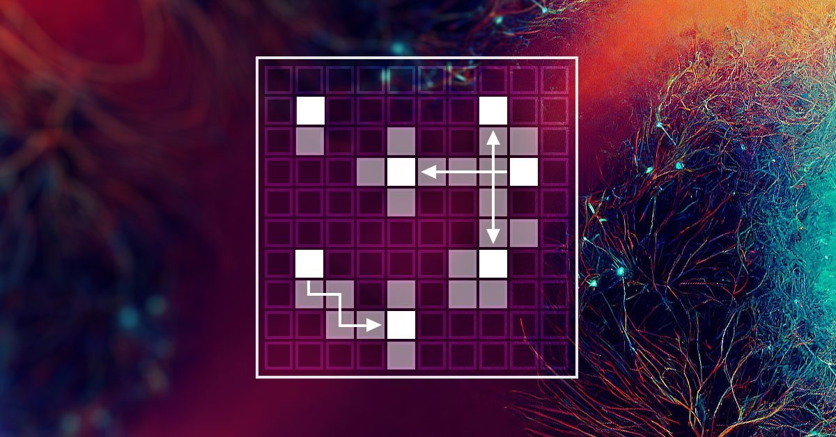
To find the coefficients of dependence between the elements of the sequence, we need to multiply in pairs the embedding of each sequence element from the Query tensor by the embeddings of all elements from the Key tensor (including the embedding of the corresponding element). When using matrix operations, we can simply multiply the Query matrix by the transposed Key matrix.
![]()
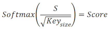
We divide the obtained values by the square root of the Key embedding dimension and normalize using the Softmax function in the context of the Query embedding sequence elements. As a result of this operation, we get a square matrix of dependencies between the elements of the initial data sequence.
Pay attention to the following two points:
- By using the Softmax function we got normalized dependency coefficient in the range 0 to 1. In this case, the row-wise sum of the coefficients is equal to 1.
- We used different matrices to create the Query and Key embeddings. This means that we got different embeddings for the same element of the source data sequence. With this approach, we eventually obtain a non-diagonal matrix of dependency coefficients. In this matrix, the dependence coefficient of the A element on the B element and the inverse dependence coefficient of the B element on the A element will differ.
Let us remember the purpose of this action. As mentioned above, we would like to get a model that can build graphs of dependencies between various objects and events. We describe each object or event using feature vectors in the initial data tensor. The resulting matrix of dependence coefficients is a tabular representation of the desired graph. In this matrix, the zero values of the coefficients indicate the absence of links between the corresponding nodes of the source data. Non-zero values determine the weighted influence of one node on the value of another.
But back to the Self Attention algorithm. We multiply the obtained dependence coefficients by the corresponding embeddings in the Value tensor. We sum the resulting values of "weighted" embeddings and the resulting vector is the output of the Self Attention block for the analyzed element of the sequence. When using matrix operations, we simply use the matrix multiplication function. By multiplying a square matrix of dependency coefficients by the Value tensor we get the desired tensor of the Self Attention block results.
![]()
The Self-Attention algorithm is described above for a simple one attention head case. However, in practice we mainly use the multi-head attention option. In such an implementation, one more dimensionality reduction matrix is added. It reduces the dimension of the concatenated tensor from all attention heads to the dimension of the source data.
At the end of the Self Attention algorithm, we add the source data tensor with the attention block and then normalize the resulting value.
As you can see, tensors at the input and output of the Self Attention block are the same size. But the output tensor contains normalized values, so that the features that have a significant impact on the result are maximized. On the contrary, the value of features that do not affect the result and noise phenomena will be minimized. Usually, several subsequent attention blocks are used in models to enhance this effect.
However, the attention block can only help us find the significant features. It does not provide a solution to the problem. Therefore, the attention block is followed by a decision-making block. This block can be a fully connected perceptron or any previously studied architectural solution.
2. Implementation using MQL5
Now that we move on to the implementation, it should be noted that we will not repeat the model from the original article "Deep reinforcement learning with relational inductive biases". We will use the suggested developments and will add a relational module to our model using the internal curiosity module. We have created a copy of this model in the previous article. Let us create a copy of the Expert Advisor from the previous article and save it as RLL-Learning.mq5.
Changing the internal architecture of the model we are training without changing the source data layer and the result layer does not require changing the EA algorithm, and thus we could simply create new model files without making changes directly to the EA code. However, in the comments to previously published articles, I often receive messages about errors in loading the models created using the NetCreator tool. Therefore, in this article, I decided to get back to compiling the model architecture description in the EA code.
Of course, you can still use NetCreator to create the necessary models. But in this case, you should pay attention to the following.
In the EA code, the model name is specified by a macro substitution. Therefore, the model should correspond to the specified format.
#define FileName Symb.Name()+"_"+EnumToString(TimeFrame)+"_"+StringSubstr(__FILE__,0,StringFind(__FILE__,".",0))
The file name is made up of:
- The symbol of the chart on which the EA is running. It is the full name of the symbol as it appears in your terminal, including prefixes and suffixes.
- Timeframe specified in the EA parameters.
- EA file name without extension.
All of the above components are separated by an underscore.
One of the following extensions is added to the file name:
- "nnw" for a model being trained
- "fwd" for Forward Model,
- "inv" for Inverse Model.
Save all the files of the created models in the "Files" directory of your terminal or in "Common/Files". In this case, the directory with the files must match the common flag specified in the program code. The true value of the common flag corresponds to the "Common/Files" directory.
bool CNet::Load(string file_name, float &error, float &undefine, float &forecast, datetime &time, bool common = true)
Now let us get back to the code of our Expert Advisor. In the OnInit function, we first initialize classes for working with indicators.
//+------------------------------------------------------------------+
//| Expert initialization function                                   |
//+------------------------------------------------------------------+
int OnInit()
  {
//---
   if(!Symb.Name(_Symbol))
      return INIT_FAILED;
   Symb.Refresh();
//---
   if(!RSI.Create(Symb.Name(), TimeFrame, RSIPeriod, RSIPrice))
      return INIT_FAILED;
//---
   if(!CCI.Create(Symb.Name(), TimeFrame, CCIPeriod, CCIPrice))
      return INIT_FAILED;
//---
   if(!ATR.Create(Symb.Name(), TimeFrame, ATRPeriod))
      return INIT_FAILED;
//---
   if(!MACD.Create(Symb.Name(), TimeFrame, FastPeriod, SlowPeriod, SignalPeriod, MACDPrice))
      return INIT_FAILED;
Then we try to load the previously prepared models. Please note that I am loading models from the "Common/Files" directory. This approach allows me to use the EA without changes both in the Strategy Tester and in real time. This is because when the EA is launched in the Strategy Tester, it does not access the terminal's "Files" directory. For security reasons, the Strategy Tester creates "its own sandbox" for each testing agent. However, each agent has access to the shared file resource, i.e. the "Common/Files" directory.
//---
   if(!StudyNet.Load(FileName + ".icm", true))
      if(!StudyNet.Load(FileName + ".nnw", FileName + ".fwd", FileName + ".inv", 6, true))
        {
If pre-trained models fail to load, we create a description of the architecture of the models used. I implemented this subprocess into a separate CreateDescriptions method. Here we call it and check the result of the operations. In case of failure, we delete unnecessary objects and exit the EA initialization function with the INIT_FAILED result.
         CArrayObj *model = new CArrayObj();
         CArrayObj *forward = new CArrayObj();
         CArrayObj *inverse = new CArrayObj();
         if(!CreateDescriptions(model, forward, inverse))
           {
            delete model;
            delete forward;
            delete inverse;
            return INIT_FAILED;
           }
After successfully creating the description of all three required models, we call the model creation method. Make sure to check the operation execution result.
         if(!StudyNet.Create(model, forward, inverse))
           {
            delete model;
            delete forward;
            delete inverse;
            return INIT_FAILED;
           }
         StudyNet.SetStateEmbedingLayer(6);
         delete model;
         delete forward;
         delete inverse;
        }
Next, we specify the neural layer of the model we are training with the encoder results and delete the architecture description objects of the created models that are no longer needed.
In the next step, we will switch the model into training mode and specify the size of the experience replay buffer.
   if(!StudyNet.TrainMode(true))
      return INIT_FAILED;
   StudyNet.SetBufferSize(Batch, 10 * Batch);
Let's set the sizes of indicator buffers.
//---
   CBufferFloat* temp;
   if(!StudyNet.GetLayerOutput(0, temp))
      return INIT_FAILED;
   HistoryBars = (temp.Total() - 9) / 12;
   delete temp;
   if(!RSI.BufferResize(HistoryBars) || !CCI.BufferResize(HistoryBars) ||
      !ATR.BufferResize(HistoryBars) || !MACD.BufferResize(HistoryBars))
     {
      PrintFormat("%s -> %d", __FUNCTION__, __LINE__);
      return INIT_FAILED;
     }
Specify the trade operations execution type.
//---
   if(!Trade.SetTypeFillingBySymbol(Symb.Name()))
      return INIT_FAILED;
//---
   return(INIT_SUCCEEDED);
  }
This completes the EA initialization method. Now we move on to the CreateDescriptions method which creates a description of the model architecture.
bool CreateDescriptions(CArrayObj *Description, CArrayObj *Forward, CArrayObj *Inverse)
  {
In the parameters, this method receives pointers to three dynamic arrays to write the architectures of the three models:
- Description — model being trained,
- Forward model,
- Inverse model.
In the method body, we immediately check the received pointers. If necessary, we create new object instances.
//---
   if(!Description)
     {
      Description = new CArrayObj();
      if(!Description)
         return false;
     }
//---
   if(!Forward)
     {
      Forward = new CArrayObj();
      if(!Forward)
         return false;
     }
//---
   if(!Inverse)
     {
      Inverse = new CArrayObj();
      if(!Inverse)
         return false;
     }
We again control the operation execution process. In case of failure, we complete the method with the False result.
After successfully creating the necessary objects, we move on to the next subprocess in which we describe the architecture of the models being created. We start with the architecture of the training model. We clear the dynamic array to write the description of the model architecture and prepare a variable to write a pointer to one neural layer description object ClayerDescription.
//--- Model
   Description.Clear();
   CLayerDescription *descr;
As usual, we first create the neural layer of the source data. As an input data layer, we will use a fully connected neural layer without an activation function. We specify the size of the neural layer equal to the number of values transferred to the model. Note that to describe each historical data candlestick, we transfer 12 values. These are the description of the candlestick and the values of the analyzed indicators. In addition, we pass the account status and the volume of open positions. Which adds 9 more values.
The neural layer description algorithm will be repeated for each neural layer. It consists of three steps. First, we create a new instance of the neural layer description object. Do not forget to check the operation result, since if there is an error in creating a new object, we can get a critical error accessing a non-existent object.
Next, we set the description of the neural layer. Here, the number of specified parameters varies depending on the type of neural layer. For the input data layer, we specify the neural layer type, the number of elements in the neural layer, the parameter optimization type and the activation function.
After specifying all the necessary parameters of the neural layer, we add a pointer to the neural layer description object to the dynamic array of the model architecture description.
//--- Input layer
   if(!(descr = new CLayerDescription()))
      return false;
   descr.type = defNeuronBaseOCL;
   int prev_count = descr.count = HistoryBars * 12 * 9;
   descr.window = 0;
   descr.activation = None;
   descr.optimization = ADAM;
   if(!Description.Add(descr))
     {
      delete descr;
      return false;
     }
According to my experience in training neural networks, the learning process is more stable when using normalized initial data. To normalize data during training and usage, we will use a batch normalization layer. We will create it right after the source data layer.
Here, again, we first create a new instance of the neural layer description object and check the result of the operation. Next, specify the type of neural layer to be created - defNeuronBatchNormOCL, the number of elements at the size level of the previous neural layer. and the normalization batch size. After that, we add a pointer to the object of the description of the neural layer to the dynamic array of the model architecture description.
//--- layer 1
   if(!(descr = new CLayerDescription()))
      return false;
   descr.type = defNeuronBatchNormOCL;
   descr.count = prev_count;
   descr.batch = 1000;
   descr.activation = None;
   descr.optimization = ADAM;
   if(!Description.Add(descr))
     {
      delete descr;
      return false;
     }
After normalizing the data, we will create a preprocessing block. Here we will use convolutional neural layers to find patterns in the source data.
As before, we create a new instance of the ClayerDescription neural layer description object, specify the defNeuronConvOCL neural layer type, specify the window of analyzed data equal to 3 elements and set the data window step to 1. With these parameters, the number of elements in one filter will be by 2 less than the size of the previous layer. To maximize the potential, I created 16 filters in this neural layer. This seems to be too many filters, but I wanted to make the model as flexible as possible. I used LeakReLU as an activation function. To optimize parameters, we will use Adam.
//--- layer 2
   if(!(descr = new CLayerDescription()))
      return false;
   descr.type = defNeuronConvOCL;
   descr.count = prev_count - 2;
   descr.window = 3;
   descr.step = 1;
   descr.window_out = 16;
   descr.activation = LReLU;
   descr.optimization = ADAM;
   if(!Description.Add(descr))
     {
      delete descr;
      return false;
     }
The next step is not standard. After the convolutional layer, we usually used a subsampling layer for dimensionality reduction. But this time we work with time series. In addition to the values, we need to track the feature change dynamics. To do this, I decided to conduct an experiment and use an LSTM block after the convolutional layer. Of course, its size will be less than the output of the convolutional layer. But because of the architecture of the recurrent block, we expect to get a dimensionality reduction considering the previous states of the system.
//--- layer 3
   if(!(descr = new CLayerDescription()))
      return false;
   descr.type = defNeuronLSTMOCL;
   descr.count = 300;
   descr.optimization = ADAM;
   if(!Description.Add(descr))
     {
      delete descr;
      return false;
     }
To reveal more complex structures, we will repeat the block of convolutional and recurrent neural layers.
//--- layer 4
   if(!(descr = new CLayerDescription()))
      return false;
   descr.type = defNeuronConvOCL;
   descr.count = 100;
   descr.window = 3;
   descr.step = 3;
   descr.window_out = 10;
   descr.activation = LReLU;
   descr.optimization = ADAM;
   if(!Description.Add(descr))
     {
      delete descr;
      return false;
     }

//--- layer 5
   if(!(descr = new CLayerDescription()))
      return false;
   descr.type = defNeuronLSTMOCL;
   descr.count = 100;
   descr.optimization = ADAM;
   if(!Description.Add(descr))
     {
      delete descr;
      return false;
     }
Next we move on to the relational block of our training model. Here we will use a block from a multilayer multi-head Self Attention. To do this, we specify the defNeuronMLMHAttentionOCL neural layer type. The number of elements of the initial data sequence will be equal to the number of analyzed candles. In this case, the number of one candlestick description features will be 5.
Do not confuse the number of signs describing one candlestick at the model input and at the input of the relational block. Since the relational block was preceded by data preprocessing performed by convolutional and recurrent neural layers.
The Keys vector size will be equal to 16. The number of heads will be equal to 64. Similarly to the filters of convolutional neural networks, I indicated a higher number of attention heads in order to comprehensively analyze the current market situation.
We will create four such layers. But we will not save this neural layer description four times. Instead, we will set the layers parameter equal to 4.
As in all previous cases, we will use the Adam method for optimizing parameters. We do not specify the activation function in this case since all activation functions are indicated by the neural layer construction algorithm.
//--- layer 6
   if(!(descr = new CLayerDescription()))
      return false;
   descr.type = defNeuronMLMHAttentionOCL;
   descr.count = 20;
   descr.window = 5;
   descr.step = 64;
   descr.window_out = 16;
   descr.layers = 4;
   descr.optimization = ADAM;
   if(!Description.Add(descr))
     {
      delete descr;
      return false;
     }
To complete the description of the model architecture, we need to indicate the layer of the fully parameterized quantile function. In the description of this neural layer, we indicate only the neural layer type defNeuronFQF, the action space, the number of quantiles and the parameter optimization method.
//--- layer 7
   if(!(descr = new CLayerDescription()))
      return false;
   descr.type = defNeuronFQF;
   descr.count = 4;
   descr.window_out = 32;
   descr.optimization = ADAM;
   if(!Description.Add(descr))
     {
      delete descr;
      return false;
     }
This concludes the sub-process related to describing the architecture of the training model. Now we need Forward and Inverse models. We will use their architecture from the previous article. For the Expert Advisor to work properly, we need to add their description into our method. The description sub-process is identical to the process described above.
First, we clear the dynamic array of the Forward model architecture description. Then we add the source data neural layer. For the Forward model, the size of the input data layer is equal to the concatenated vector from the size of the main model's encoder output and the space of possible agent actions.
//--- Forward
   Forward.Clear();
//--- Input layer
   if(!(descr = new CLayerDescription()))
      return false;
   descr.type = defNeuronBaseOCL;
   descr.count = 104;
   descr.window = 0;
   descr.activation = None;
   descr.optimization = ADAM;
   if(!Forward.Add(descr))
     {
      delete descr;
      return false;
     }
This is followed by a fully connected neural layer of 500 elements with the LReLU activation function and the Adam optimization method.
//--- layer 1
   if(!(descr = new CLayerDescription()))
      return false;
   descr.type = defNeuronBaseOCL;
   descr.count = 500;
   descr.activation = LReLU;
   descr.optimization = ADAM;
   if(!Forward.Add(descr))
     {
      delete descr;
      return false;
     }
At the output of the Forward block, we expect to get the next state at the model encoder output. Therefore, this model is completed by a fully connected neural layer, in which the number of neurons is equal to the size of the vector at the model encoder output. No activation function is used. Again, we use Adam for the parameter optimization method.
//--- layer 2
   if(!(descr = new CLayerDescription()))
      return false;
   descr.type = defNeuronBaseOCL;
   descr.count = 100;
   descr.activation = None;
   descr.optimization = ADAM;
   if(!Forward.Add(descr))
     {
      delete descr;
      return false;
     }
The Inverse model construction approach is similar. The only difference is that we feed the concatenated vector of two subsequent states into this block. Therefore, the size of the source data layer is twice the size of the model encoder output.
//--- Inverse
   Inverse.Clear();
//--- Input layer
   if(!(descr = new CLayerDescription()))
      return false;
   descr.type = defNeuronBaseOCL;
   descr.count = 200;
   descr.window = 0;
   descr.activation = None;
   descr.optimization = ADAM;
   if(!Inverse.Add(descr))
     {
      delete descr;
      return false;
     }
The second neural layer is the same as that of the Forward model.
//--- layer 1
   if(!(descr = new CLayerDescription()))
      return false;
   descr.type = defNeuronBaseOCL;
   descr.count = 500;
   descr.activation = LReLU;
   descr.optimization = ADAM;
   if(!Inverse.Add(descr))
     {
      delete descr;
      return false;
     }
We expect the taken action at the output of the Inverse model. Therefore, the size of the next neural layer is equal to the space of possible agent actions. This layer does not use the activation function. We will use the next Softmax layer instead.
//--- layer 2
   if(!(descr = new CLayerDescription()))
      return false;
   descr.type = defNeuronBaseOCL;
   descr.count = 4;
   descr.activation = None;
   descr.optimization = ADAM;
   if(!Inverse.Add(descr))
     {
      delete descr;
      return false;
     }
//--- layer 3
   if(!(descr = new CLayerDescription()))
      return false;
   descr.type = defNeuronSoftMaxOCL;
   descr.count = 4;
   descr.step = 1;
   descr.activation = None;
   descr.optimization = ADAM;
   if(!Inverse.Add(descr))
     {
      delete descr;
      return false;
     }
//---
   return true;
  }
The remaining EA code is the same that we considered in the previous article. The complete EA code and all the libraries used are provided in the attachment.
3. Test
The model was trained and tested in the Strategy Tester using the EURUSD historical data, with the H1 timeframe. Indicators were used with default parameters.

The model training showed the balance growth in the Strategy Tester. Although there are 2 losing trades per every 2 profitable trades on average, the share of profitable trades was 53.7%. In general, we see a fairly even increase in the balance and equity graphs, as the average profitable trade is 12.5% higher than the average losing one. The profit factor is 1.31, and the recovery factor is 2.85.


Conclusion
In this article, we got acquainted with the relational approaches in the field of reinforcement learning. We added a relational block to the model and trained it using the Intrinsic Curiosity Module. The test results confirmed the feasibility of this approach to model training. These models can be used as the basis in creating EAs that are capable of generating profit.
Although the presented EA can perform trading operations, it is not ready for use in real trading. The EA is presented for evaluation purposes only. Significant refinement and comprehensive testing in all possible conditions are required before real life use.
List of references
- Neural Machine Translation by Jointly Learning to Align and Translate
- Effective Approaches to Attention-based Neural Machine Translation
- Attention Is All You Need
- Deep reinforcement learning with relational inductive biases
- Neural networks made easy (Part 8): Attention mechanisms
- Neural networks made easy (Part 10): Multi-Head Attention
- Neural networks made easy (Part 11): A take on GPT
- Neural networks made easy (Part 35): Intrinsic Curiosity Module
Programs used in the article
| # | Name | Type | Description |
|---|---|---|---|
| 1 | RRL-learning.mq5 | Expert Advisor | Model training EA |
| 2 | ICM.mqh | Class library | Model organization class library |
| 3 | NeuroNet.mqh | Class library | A library of classes for creating a neural network |
| 4 | NeuroNet.cl | Code Base | OpenCL program code library |
Translated from Russian by MetaQuotes Ltd.
Original article: https://www.mql5.com/ru/articles/11876
Warning: All rights to these materials are reserved by MetaQuotes Ltd. Copying or reprinting of these materials in whole or in part is prohibited.
This article was written by a user of the site and reflects their personal views. MetaQuotes Ltd is not responsible for the accuracy of the information presented, nor for any consequences resulting from the use of the solutions, strategies or recommendations described.

- Free trading apps
- Over 8,000 signals for copying
- Economic news for exploring financial markets
You agree to website policy and terms of use
Hi Dmitry Gizlyk,
Thanks for your wonderful articles.
Please help! When I try to train in Strategy Tester using Ryzen 9 6900hx (APU), I got this error and the EA had no transaction.
How to fix this problem bro?
Hi Dmitry,
Thank you for the awesome work! This is the best tutorial so far on the net regarding ML on MQL5 platform
Details are well explained and can be understood by new learner.
Following your tutorial, I've run Strategy Tester and apparently, only one of my processors were used despite there are 12 available as shown in the picture below
Is there any way to activate all cores instead of just one?
OS Windows 11 build 22H2
OpenCL Support 3.0
CPU Intel i5-12400 ghz.html)
GPU Intel UHD Graphic 730 (integrated)
RAM 16gb
OpenCL are already enabled in Metatrader's settings.
Thanks for the detailed tutorial!
Hi, at Strategy tester you can see only one core use. It used by mql programme, not OpenCL. OpenCL use GPU or CPU cores in system outside Strategy tester monitor. There are several ways to see the resource consumption of an OpenCL programme in Windows:
1. Use performance monitoring software such as MSI Afterburner or GPU-Z, which display GPU usage and other system components. They can also show what portion of resources each OpenCL program is using.
2. Use profilers such as AMD CodeXL or NVIDIA Nsight Visual Studio Edition. They allow you to analyse an OpenCL program and display which parts of the code consume the most time and resources.
3. Use the OpenCL API to gather statistics. This allows you to programmatically obtain information about the use of OpenCL resources, such as memory usage or core performance. You can use the Performance Counters for OpenCL (PCPerfCL) library to gather this information in Windows.
4. Use profiling tools such as Intel VTune Amplifier, which can help you see how a program uses processor and other system component resources.
Good afternoon Dimitri!
Please help me to run your Expert Advisor from this article. I have tried everything to make it work, but alas it does not work properly.
The problem is as follows: the Expert Advisor starts in the tester and begins the test in the tester normally, counting down the seconds, green bar, no errors in the log, normally sees the video card and selects it. But there is 0% load on the video card. It's like it's not counting anything on it. In Common\Files there are 2 files with extensions icm and nnw with size 1 kb. When I try to restart the test in the tester again, it warns that it cannot initialise and the test does not start. If you restart MT5 and delete the files created by this EA in Common\Files, it starts normally, but also does not use the video card and creates again these files of 1 kb. and so on and so forth.
I tried to take NeuroNet.mqh files from the next article (that you posted there in the comments) and replace the one in the article with it - it didn't help. I tried selecting a small time period in the tester (1 month, 1 week, 2 months, etc.) also didn't help.
How to start it? The Expert Advisors from previous articles run normally and use the video card correctly.
There is also a problem with the Expert Advisor from the next article 37, 38. On the contrary, there is no progress in the tester, but the video card is used to the maximum and so at least 5 hours, even 10 hours.
The Expert Advisor from article 39 worked fine. There I chose the history of more than 1 month and it did not create the database, but I chose 1 month and it created the database normally. The rest of its parts worked normally.
This is a real gem, Dmitriy!
I am a data scientist with hands-on developing various machine learning algorithms on time-series data, and yet I find your series informative and well-written. This is a valuable basis to build on.
Thank you for sharing your work.
Bijan