
Neural networks made easy (Part 68): Offline Preference-guided Policy Optimization

Introduction
Reinforcement learning is a universal platform for learning optimal behavior policies in the environment under exploration. Policy optimality is achieved by maximizing the rewards received from the environment during interaction with it. But herein lies one of the main problems of this approach. The creation of an appropriate reward function often requires significant human effort. Additionally, rewards may be sparse and/or insufficient to express the true learning goal. As one of the options for solving this problem, the authors if the paper "Beyond Reward: Offline Preference-guided Policy Optimization" suggested the OPPO method (OPPO stands for the Offline Preference-guided Policy Optimization). The authors of the method suggest the replacement of the reward given by the environment with the preferences of the human annotator between two trajectories completed in the environment under exploration. Let's take a closer look at the proposed algorithm.
1. The OPPO algorithm
In the context of offline preference-guided learning, the general approach consists of two steps and typically involves optimizing the reward function model using supervised learning, and then training the policy using any offline RL algorithm on transitions redefined using the learned reward function. However, the practice of separate training of the reward function may not directly instruct the policy how to act optimally. The preference labels define the learning task, and thus the goal is to learn the most preferred trajectory rather than to maximize the reward. In cases of complex problems, scalar rewards can create an information bottleneck in policy optimization, which in turn leads to suboptimal behavior of the Agent. Additionally, offline policy optimization can exploit vulnerabilities in incorrect reward functions. This in turn leads to unwanted behavior.
As an alternative to this two-step approach, the authors of the Offline Preference-guided Policy Optimization method (OPPO) aim to learn policy directly from an offline preference-guided dataset. They propose a one-step algorithm that simultaneously models offline preferences and learns the optimal decision policy without the need to separately train the reward function. This is achieved through the use of two goals:
- Collating information "in the absence" of offline;
- Preference modeling.
By iteratively optimizing these goals, we come to the construction of a contextual policy π(A|S,Z) to model offline data and optimal context of preferences Z'. OPPO's focus is on exploring high-dimensionality space Z and evaluating the policy in such a space. This high-dimensional Z-space captures more information about the task at hand compared to a scalar payoff, making it ideal for policy optimization purposes. In addition, the optimal policy is obtained by conditionally modeling the contextual policy π(A|S,Z) on the learned optimal context Z'.
The authors of the algorithm introduce the assumption that it is possible to approximate the preference function by the model Iθ, which allows us to formulate the following goal:
![]()
where Z=Iθ(τ) is the context of preferences. This encoder-decoder structure will resemble offline simulation learning. However, since the preference-based learning setting lacks expert demonstrations, the authors of the algorithm use preference labels to extract retrospective information.
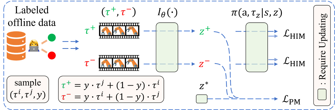
To achieve consistency with historical information Iθ(τ) and preferences in a labeled data set, the authors of the method formulate the following goal of preference modeling:
![]()
where z+ and z- represent the context of the preferred (positive) trajectory Iθ(yτj + (1-y)τi) and less preferable (negative) trajectory Iθ(yτi + (1-y)τj), respectively. The underlying assumption in this goal is that people typically make two-level comparisons before expressing preferences between two trajectories (τi, τj):
- Separate comparison of similarity between trajectory τi and a hypothetical optimal trajectory τ*, that is l(z*,z+) and of similarity between trajectory τj and a hypothetical optimal trajectory τ*, that is l(z*,z-),
- Estimate of differences between these two similarities l(z*,z+) and l(z*,z-) with the trajectory set to the one closer to the preferred one.
Thus, goal optimization ensures that an optimal context is found that is more similar to z+ and less similar to z-.
It should be clarified that z* is the relevant context for the trajectory τ*, while the trajectory τ* will always be preferred over any offline trajectories in the dataset.
Note that the posterior probability of the optimal context z* and the extraction of retrospective preference information Iθ(•) are updated one by one to ensure training stability. A better estimate of the optimal embedding helps the encoder to extract features that a person pays more attention to when determining preferences. In turn, a better retrospective information encoder speeds up the process of finding the optimal trajectory in the high-level embedding space. Thus, the loss function for the encoder consists of two parts:
- Error in comparing information from retrospectives in the supervised training style.
- Error to better incorporate the binary observation provided by the labeled preference dataset.
The authors' visualization of the OPPO algorithm is presented below.
2. Implementation using MQL5
We have considered the theoretical aspects of the algorithms, so now let us move on to the practical part, in which we will consider the implementation of the proposed algorithm. We will start with the data storage structure SState. As mentioned above, the authors of the method replace the traditionally used reward with a trajectory preference label. Therefore, we do not need to save rewards at each transition to a new state of the environment. At the same time, we introduce the concept of preferred trajectory context. Following the proposed logic in the environment state description structure, we replace the rewards array with decomposed rewards with the scheduler context array.
struct SState
  {
   float             state[BarDescr * NBarInPattern];
   float             account[AccountDescr];
   float             action[NActions];
   float             scheduler[EmbeddingSize];
   //---
                     SState(void);
   //---
   bool              Save(int file_handle);
   bool              Load(int file_handle);
   //---
   void              Clear(void)
     {
      ArrayInitialize(state, 0);
      ArrayInitialize(account, 0);
      ArrayInitialize(action, 0);
      ArrayInitialize(scheduler, 0);
     }
   //--- overloading
   void              operator=(const SState &obj)
     {
      ArrayCopy(state, obj.state);
      ArrayCopy(account, obj.account);
      ArrayCopy(action, obj.action);
      ArrayCopy(scheduler, obj.scheduler);
     }
  };
Please note that we changed not only the name, but also the size of the array.
In addition to the hidden context, the algorithm also introduces the concept of trajectory preference. There are several aspects to pay attention to here:
- Priority is set for the trajectory as a whole, rather than individual actions and transitions (policy is assessed).
- Priorities are set in pairs between all trajectories in the offline data set in the range [0: 1].
- Priorities are set by an expert.
Please note that we will not manually set priorities to all trajectories from the experience replay buffer. Also, we will not make a chess table of priorities.
There are quite a lot of priority criteria that can be chosen. But within the framework of this article, I used only one which is the profit from passing the trajectory. I agree that we could add the maximum drawdown in terms of both balance and Equity to the criteria. Also, we could add the profit factor and other criteria. However, I suggest you independently choose the optimal set of criteria for you and their value coefficients. The set of criteria you choose will certainly affect the final result of policy training but will not affect the algorithm of the proposed implementation.
And since priority is set for the trajectory as a whole, we only need to save the amount of profit received at the end of the trajectory. We will save it in the trajectory description structure STrajectory.
struct STrajectory
  {
   SState            States[Buffer_Size];
   int               Total;
   double            Profit;
   //---
                     STrajectory(void);
   //---
   bool              Add(SState &state);
   void              ClearFirstN(const int n);
   //---
   bool              Save(int file_handle);
   bool              Load(int file_handle);
   //--- overloading
   void              operator=(const STrajectory &obj)
     {
      Total = obj.Total;
      Profit = obj.Profit;
      for(int i = 0; i < Buffer_Size; i++)
         States[i] = obj.States[i];
     }
  };
Of course, changing the fields of structures will require changes to the methods of copying and working with files of the specified structures. But these adjustments are so specific that I suggest you familiarize yourself with them in the attached files.
2.1 Model architecture
We will use 2 models to train the policy. The Scheduler will learn preferences, and the Agent will learn behavior policies. Both models will be built on the principle of Decision Transformer (DT) and use attention mechanisms. However, unlike the authors' solution to update models one by one, we will create 2 Expert Advisors for training models. Each of them will participate in the training of only one model. We will combine them into a single mechanism at the stage of testing and operating the model. Therefore, to describe the architecture of the models, we will also create 2 methods:
- CreateSchedulerDescriptions - to describe the Scheduler architecture
- CreateAgentDescriptions - to describe the Agent architecture
We will input into the Scheduler the following:
- Historical price movement and indicator data
- Descriptions of account status and open positions
- Timestamp
- Last action of the Agent
bool CreateSchedulerDescriptions(CArrayObj *scheduler)
  {
//---
   CLayerDescription *descr;
//---
   if(!scheduler)
     {
      scheduler = new CArrayObj();
      if(!scheduler)
         return false;
     }
//--- Scheduler
   scheduler.Clear();
//--- Input layer
   if(!(descr = new CLayerDescription()))
      return false;
   descr.type = defNeuronBaseOCL;
   int prev_count = descr.count = (BarDescr * NBarInPattern +
                                   AccountDescr + TimeDescription + NActions);
   descr.activation = None;
   descr.optimization = ADAM;
   if(!scheduler.Add(descr))
     {
      delete descr;
      return false;
     }
As we have seen in earlier articles, the Decision Transformer exploits the GPT architecture and stores embeddings of previously received data in its hidden state, which allows you to make decisions in a single context throughout the entire episode. Therefore, we feed only a brief description of the current state to the model, focusing on the latest changes. In other words, we input only data about the last closed candlestick into the model.
The received data is preprocessed in the normalization layer.
//--- layer 1
   if(!(descr = new CLayerDescription()))
      return false;
   descr.type = defNeuronBatchNormOCL;
   descr.count = prev_count;
   descr.batch = 1000;
   descr.activation = None;
   descr.optimization = ADAM;
   if(!scheduler.Add(descr))
     {
      delete descr;
      return false;
     }
After which, it is converted into a comparable form in the Embedding layer.
//--- layer 2
   if(!(descr = new CLayerDescription()))
      return false;
   descr.type = defNeuronEmbeddingOCL;
   prev_count = descr.count = HistoryBars;
     {
      int temp[] = {BarDescr * NBarInPattern, AccountDescr, TimeDescription, NActions};
      ArrayCopy(descr.windows, temp);
     }
   int prev_wout = descr.window_out = EmbeddingSize;
   if(!scheduler.Add(descr))
     {
      delete descr;
      return false;
     }
We then normalize the resulting embeddings using the SoftMax function.
//--- layer 3
   if(!(descr = new CLayerDescription()))
      return false;
   descr.type = defNeuronSoftMaxOCL;
   descr.count = EmbeddingSize;
   descr.step = prev_count * 4;
   descr.activation = None;
   descr.optimization = ADAM;
   if(!scheduler.Add(descr))
     {
      delete descr;
      return false;
     }
The data preprocessed in this way passes through the attention block.
//--- layer 4
   if(!(descr = new CLayerDescription()))
      return false;
   descr.type = defNeuronMLMHAttentionOCL;
   prev_count = descr.count = prev_count * 4;
   descr.window = EmbeddingSize;
   descr.step = 8;
   descr.window_out = 32;
   descr.layers = 4;
   descr.optimization = ADAM;
   if(!scheduler.Add(descr))
     {
      delete descr;
      return false;
     }
We again normalize the received data with the SoftMax function and pass it through a block of fully connected decision layers.
//--- layer 5
   if(!(descr = new CLayerDescription()))
      return false;
   descr.type = defNeuronSoftMaxOCL;
   descr.count = EmbeddingSize;
   descr.step = prev_count;
   descr.activation = None;
   descr.optimization = ADAM;
   if(!scheduler.Add(descr))
     {
      delete descr;
      return false;
     }
//--- layer 6
   if(!(descr = new CLayerDescription()))
      return false;
   descr.type = defNeuronBaseOCL;
   descr.count = LatentCount;
   descr.optimization = ADAM;
   descr.activation = LReLU;
   if(!scheduler.Add(descr))
     {
      delete descr;
      return false;
     }
//--- layer 7
   if(!(descr = new CLayerDescription()))
      return false;
   descr.type = defNeuronBaseOCL;
   prev_count = descr.count = EmbeddingSize;
   descr.activation = None;
   descr.optimization = ADAM;
   if(!scheduler.Add(descr))
     {
      delete descr;
      return false;
     }
//---
   return true;
  }
At the output of the model, we receive a vector of latent representation of the context, the size of which is determined by the EmbeddingSize constant.
We are drawing a similar architecture for our Agent. The generated context is added in its source data.
//+------------------------------------------------------------------+
//|                                                                  |
//+------------------------------------------------------------------+
bool CreateAgentDescriptions(CArrayObj *agent)
  {
//---
   CLayerDescription *descr;
//---
   if(!agent)
     {
      agent = new CArrayObj();
      if(!agent)
         return false;
     }
//--- Agent
   agent.Clear();
//--- Input layer
   if(!(descr = new CLayerDescription()))
      return false;
   descr.type = defNeuronBaseOCL;
   int prev_count = descr.count = (BarDescr * NBarInPattern +
                                   AccountDescr + TimeDescription +
                                   NActions + EmbeddingSize);
   descr.activation = None;
   descr.optimization = ADAM;
   if(!agent.Add(descr))
     {
      delete descr;
      return false;
     }
The data is also preprocessed through batch normalization and embedding layers and is normalized by the SoftMax function.
//--- layer 1
   if(!(descr = new CLayerDescription()))
      return false;
   descr.type = defNeuronBatchNormOCL;
   descr.count = prev_count;
   descr.batch = 1000;
   descr.activation = None;
   descr.optimization = ADAM;
   if(!agent.Add(descr))
     {
      delete descr;
      return false;
     }
//--- layer 2
   if(!(descr = new CLayerDescription()))
      return false;
   descr.type = defNeuronEmbeddingOCL;
   prev_count = descr.count = HistoryBars;
     {
      int temp[] = {BarDescr * NBarInPattern, AccountDescr,
                    TimeDescription, NActions, EmbeddingSize};
      ArrayCopy(descr.windows, temp);
     }
   int prev_wout = descr.window_out = EmbeddingSize;
   if(!agent.Add(descr))
     {
      delete descr;
      return false;
     }
//--- layer 3
   if(!(descr = new CLayerDescription()))
      return false;
   descr.type = defNeuronSoftMaxOCL;
   descr.count = EmbeddingSize;
   descr.step = prev_count * 5;
   descr.activation = None;
   descr.optimization = ADAM;
   if(!agent.Add(descr))
     {
      delete descr;
      return false;
     }
We completely repeat the attention block followed by normalization with the SoftMax function. Here you should only pay attention to changing the size of the processed tensor.
//--- layer 4
   if(!(descr = new CLayerDescription()))
      return false;
   descr.type = defNeuronMLMHAttentionOCL;
   prev_count = descr.count = prev_count * 5;
   descr.window = EmbeddingSize;
   descr.step = 8;
   descr.window_out = 32;
   descr.layers = 4;
   descr.optimization = ADAM;
   if(!agent.Add(descr))
     {
      delete descr;
      return false;
     }
//--- layer 5
   if(!(descr = new CLayerDescription()))
      return false;
   descr.type = defNeuronSoftMaxOCL;
   descr.count = EmbeddingSize;
   descr.step = prev_count;
   descr.activation = None;
   descr.optimization = ADAM;
   if(!agent.Add(descr))
     {
      delete descr;
      return false;
     }
Next, we reduce the dimensionality of the data using convolutional layers and at the same time try to identify stable patterns in them.
//--- layer 6
   if(!(descr = new CLayerDescription()))
      return false;
   descr.type = defNeuronConvOCL;
   prev_count = descr.count = prev_count;
   descr.window = EmbeddingSize;
   descr.step = EmbeddingSize;
   prev_wout = descr.window_out = EmbeddingSize;
   descr.optimization = ADAM;
   descr.activation = LReLU;
   if(!agent.Add(descr))
     {
      delete descr;
      return false;
     }
//--- layer 7
   if(!(descr = new CLayerDescription()))
      return false;
   descr.type = defNeuronSoftMaxOCL;
   descr.count = prev_count;
   descr.step = prev_wout;
   descr.activation = None;
   descr.optimization = ADAM;
   if(!agent.Add(descr))
     {
      delete descr;
      return false;
     }
//--- layer 8
   if(!(descr = new CLayerDescription()))
      return false;
   descr.type = defNeuronConvOCL;
   prev_count = descr.count = prev_count;
   descr.window = prev_wout;
   descr.step = prev_wout;
   prev_wout = descr.window_out = prev_wout / 2;
   descr.optimization = ADAM;
   descr.activation = LReLU;
   if(!agent.Add(descr))
     {
      delete descr;
      return false;
     }
//--- layer 9
   if(!(descr = new CLayerDescription()))
      return false;
   descr.type = defNeuronSoftMaxOCL;
   descr.count = prev_count;
   descr.step = prev_wout;
   descr.activation = None;
   descr.optimization = ADAM;
   if(!agent.Add(descr))
     {
      delete descr;
      return false;
     }
After that the data passes through a decision-making block of 4 fully connected layers. The size of the last layer is equal to the Agent's action space.
//--- layer 10
   if(!(descr = new CLayerDescription()))
      return false;
   descr.type = defNeuronBaseOCL;
   descr.count = LatentCount;
   descr.optimization = ADAM;
   descr.activation = LReLU;
   if(!agent.Add(descr))
     {
      delete descr;
      return false;
     }
//--- layer 11
   if(!(descr = new CLayerDescription()))
      return false;
   descr.type = defNeuronBaseOCL;
   prev_count = descr.count = LatentCount;
   descr.activation = LReLU;
   descr.optimization = ADAM;
   if(!agent.Add(descr))
     {
      delete descr;
      return false;
     }
//--- layer 12
   if(!(descr = new CLayerDescription()))
      return false;
   descr.type = defNeuronBaseOCL;
   descr.count = LatentCount;
   descr.activation = LReLU;
   descr.optimization = ADAM;
   if(!agent.Add(descr))
     {
      delete descr;
      return false;
     }
//--- layer 13
   if(!(descr = new CLayerDescription()))
      return false;
   descr.type = defNeuronBaseOCL;
   descr.count = NActions;
   descr.activation = SIGMOID;
   descr.optimization = ADAM;
   if(!agent.Add(descr))
     {
      delete descr;
      return false;
     }
//---
   return true;
  }
2.2 Collecting trajectories for training
After describing the architecture of the models, we move on to constructing Expert Advisors for their training. We will start with building the EA for interaction with the environment to collect trajectories and fill the experience replay buffer, which we will later exploit in the offline learning process "...\OPPO\Research.mq5".
To explore the environment, we will use the ɛ-greedy strategy and add the corresponding external parameter to the EA.
input double Epsilon = 0.5;
As mentioned above, in the process of interaction with the environment we use both models. Therefore, we need to declare global variables for them.
CNet                 Agent;
CNet                 Scheduler;
The method of initializing the EA is not much different from the similar method of the EAs we discussed earlier. Therefore, I think there is no need to consider its algorithm again. You can check it in the attachment. Let's move on to consider the OnTick method, in the body of which the main process of interaction with the environment and data collection is built.
In the body of the method, we check for the occurrence of the event of opening a new bar.
//+------------------------------------------------------------------+
//| Expert tick function                                             |
//+------------------------------------------------------------------+
void OnTick()
  {
//---
   if(!IsNewBar())
      return;
If necessary, we download historical price movement data.
   int bars = CopyRates(Symb.Name(), TimeFrame, iTime(Symb.Name(), TimeFrame, 1),
                                                                  History, Rates);
   if(!ArraySetAsSeries(Rates, true))
      return;
Then we update the readings of the analyzed indicators.
   RSI.Refresh();
   CCI.Refresh();
   ATR.Refresh();
   MACD.Refresh();
   Symb.Refresh();
   Symb.RefreshRates();
We format the received data into the structure of the current state and transfer it to the data buffer for subsequent use as input data for our models.
//--- History data
   float atr = 0;
//---
   for(int b = 0; b < (int)NBarInPattern; b++)
     {
      float open = (float)Rates[b].open;
      float rsi = (float)RSI.Main(b);
      float cci = (float)CCI.Main(b);
      atr = (float)ATR.Main(b);
      float macd = (float)MACD.Main(b);
      float sign = (float)MACD.Signal(b);
      if(rsi == EMPTY_VALUE || cci == EMPTY_VALUE || atr == EMPTY_VALUE ||
         macd == EMPTY_VALUE || sign == EMPTY_VALUE)
         continue;
      //---
      int shift = b * BarDescr;
      sState.state[shift] = (float)(Rates[b].close - open);
      sState.state[shift + 1] = (float)(Rates[b].high - open);
      sState.state[shift + 2] = (float)(Rates[b].low - open);
      sState.state[shift + 3] = (float)(Rates[b].tick_volume / 1000.0f);
      sState.state[shift + 4] = rsi;
      sState.state[shift + 5] = cci;
      sState.state[shift + 6] = atr;
      sState.state[shift + 7] = macd;
      sState.state[shift + 8] = sign;
     }
   bState.AssignArray(sState.state);
At the next stage, we supplement the structure of the description of the current state of the environment with information about the account balance and open positions.
//--- Account description
   sState.account[0] = (float)AccountInfoDouble(ACCOUNT_BALANCE);
   sState.account[1] = (float)AccountInfoDouble(ACCOUNT_EQUITY);
//---
   double buy_value = 0, sell_value = 0, buy_profit = 0, sell_profit = 0;
   double position_discount = 0;
   double multiplyer = 1.0 / (60.0 * 60.0 * 10.0);
   int total = PositionsTotal();
   datetime current = TimeCurrent();
   for(int i = 0; i < total; i++)
     {
      if(PositionGetSymbol(i) != Symb.Name())
         continue;
      double profit = PositionGetDouble(POSITION_PROFIT);
      switch((int)PositionGetInteger(POSITION_TYPE))
        {
         case POSITION_TYPE_BUY:
            buy_value += PositionGetDouble(POSITION_VOLUME);
            buy_profit += profit;
            break;
         case POSITION_TYPE_SELL:
            sell_value += PositionGetDouble(POSITION_VOLUME);
            sell_profit += profit;
            break;
        }
      position_discount += profit - (current - PositionGetInteger(POSITION_TIME)) *
                                    multiplyer * MathAbs(profit);
     }
   sState.account[2] = (float)buy_value;
   sState.account[3] = (float)sell_value;
   sState.account[4] = (float)buy_profit;
   sState.account[5] = (float)sell_profit;
   sState.account[6] = (float)position_discount;
   sState.account[7] = (float)Rates[0].time;
The collected information is also added to the source data buffer.
   bState.Add((float)((sState.account[0] - PrevBalance) / PrevBalance));
   bState.Add((float)(sState.account[1] / PrevBalance));
   bState.Add((float)((sState.account[1] - PrevEquity) / PrevEquity));
   bState.Add(sState.account[2]);
   bState.Add(sState.account[3]);
   bState.Add((float)(sState.account[4] / PrevBalance));
   bState.Add((float)(sState.account[5] / PrevBalance));
   bState.Add((float)(sState.account[6] / PrevBalance));
Next, we add a timestamp and the Agent's last action to the source data buffer.
//--- Time label
   double x = (double)Rates[0].time / (double)(D'2024.01.01' - D'2023.01.01');
   bState.Add((float)MathSin(2.0 * M_PI * x));
   x = (double)Rates[0].time / (double)PeriodSeconds(PERIOD_MN1);
   bState.Add((float)MathCos(2.0 * M_PI * x));
   x = (double)Rates[0].time / (double)PeriodSeconds(PERIOD_W1);
   bState.Add((float)MathSin(2.0 * M_PI * x));
   x = (double)Rates[0].time / (double)PeriodSeconds(PERIOD_D1);
   bState.Add((float)MathSin(2.0 * M_PI * x));
//--- Prev action
   bState.AddArray(AgentResult);
At this stage, we have collected enough information for a feed-forward pass of the Scheduler. This will allow us to form the context vector required for our Agent. Therefore, we run the feed-forward pass of the Scheduler.
   if(!Scheduler.feedForward(GetPointer(bState), 1, false))
      return;
   Scheduler.getResults(sState.scheduler);
   bState.AddArray(sState.scheduler);
Unload the obtained result and supplement the source data buffer. After that, call the Agent's feed-forward pass method.
   if(!Agent.feedForward(GetPointer(bState), 1, false, (CBufferFloat *)NULL))
      return;
Here I would like to remind you of the need to control the correct execution of operations at each stage.
At this stage, we complete the work with the models, save the data for subsequent operations, and move on to direct interaction with the environment.
   PrevBalance = sState.account[0];
   PrevEquity = sState.account[1];
Having received data from our Agent, we add noise to it, if necessary.
   Agent.getResults(AgentResult);
   if(Epsilon > (double(MathRand()) / 32767.0))
      for(ulong i = 0; i < AgentResult.Size(); i++)
        {
         float rnd = ((float)MathRand() / 32767.0f - 0.5f) * 0.03f;
         float t = AgentResult[i] + rnd;
         if(t > 1 || t < 0)
            t = AgentResult[i] - rnd;
         AgentResult[i] = t;
        }
   AgentResult.Clip(0.0f, 1.0f);
Remove duplicate volumes from position sizes.
   double min_lot = Symb.LotsMin();
   double step_lot = Symb.LotsStep();
   double stops = MathMax(Symb.StopsLevel(), 1) * Symb.Point();
   if(AgentResult[0] >= AgentResult[3])
     {
      AgentResult[0] -= AgentResult[3];
      AgentResult[3] = 0;
     }
   else
     {
      AgentResult[3] -= AgentResult[0];
      AgentResult[0] = 0;
     }
After that, we first adjust the long position.
//--- buy control
   if(AgentResult[0] < 0.9 * min_lot || (AgentResult[1] * MaxTP * Symb.Point()) <= stops ||
      (AgentResult[2] * MaxSL * Symb.Point()) <= stops)
     {
      if(buy_value > 0)
         CloseByDirection(POSITION_TYPE_BUY);
     }
   else
     {
      double buy_lot = min_lot + MathRound((double(AgentResult[0] + FLT_EPSILON) - min_lot) /
                                                                         step_lot) * step_lot;
      double buy_tp = Symb.NormalizePrice(Symb.Ask() + AgentResult[1] * MaxTP * Symb.Point());
      double buy_sl = Symb.NormalizePrice(Symb.Ask() - AgentResult[2] * MaxSL * Symb.Point());
      if(buy_value > 0)
      TrailPosition(POSITION_TYPE_BUY, buy_sl, buy_tp);
      if(buy_value != buy_lot)
        {
         if(buy_value > buy_lot)
               ClosePartial(POSITION_TYPE_BUY, buy_value - buy_lot);
            else
               Trade.Buy(buy_lot - buy_value, Symb.Name(), Symb.Ask(), buy_sl, buy_tp);
           }
     }
And then we perform similar operations for a short position.
//--- sell control
   if(AgentResult[3] < 0.9 * min_lot || (AgentResult[4] * MaxTP * Symb.Point()) <= stops ||
      (AgentResult[5] * MaxSL * Symb.Point()) <= stops)
     {
      if(sell_value > 0)
         CloseByDirection(POSITION_TYPE_SELL);
     }
   else
     {
      double sell_lot = min_lot + MathRound((double(AgentResult[3] + FLT_EPSILON) - min_lot) /
                                                                          step_lot) * step_lot;
      double sell_tp = Symb.NormalizePrice(Symb.Bid() - AgentResult[4] * MaxTP * Symb.Point());
      double sell_sl = Symb.NormalizePrice(Symb.Bid() + AgentResult[5] * MaxSL * Symb.Point());
      if(sell_value > 0)
         TrailPosition(POSITION_TYPE_SELL, sell_sl, sell_tp);
      if(sell_value != sell_lot)
        {
         if(sell_value > sell_lot)
            ClosePartial(POSITION_TYPE_SELL, sell_value - sell_lot);
         else
            Trade.Sell(sell_lot - sell_value, Symb.Name(), Symb.Bid(), sell_sl, sell_tp);
        }
     }
At this stage, we usually form a reward vector. However, rewards are not used within the framework of the current algorithm. Therefore, we simply transfer data about the Agent's completed actions and transmit data to save the trajectory.
   for(ulong i = 0; i < NActions; i++)
      sState.action[i] = AgentResult[i];
   if(!Base.Add(sState))
      ExpertRemove();
  }
Then we move on to waiting for the next bar to open.
At this point, the following question arises: How will we evaluate preferences?
The answer is simple: We will add information about the effectiveness of the pass in the OnTester method after completing the pass in the strategy tester.
//+------------------------------------------------------------------+
//| Tester function                                                  |
//+------------------------------------------------------------------+
double OnTester()
  {
//---
   double ret = 0.0;
//---
   Base.Profit = TesterStatistics(STAT_PROFIT);
   Frame[0] = Base;
   if(Base.Profit >= MinProfit)
      FrameAdd(MQLInfoString(MQL_PROGRAM_NAME), 1, Base.Profit, Frame);
//---
   return(ret);
  }
The remaining methods of the EA for interacting with the environment remain unchanged. You can find them in the attachment. Let's move on to considering model training algorithms.
2.3 Preference Model Training
First. let's look at the preference model training EA "...\OPPO\StudyScheduler.mq5". The EA architecture has remained unchanged, so we will only consider in detail the methods involved in training the model.
I must admit that the model training process uses developments from previous articles. Symbiosis with them, in my personal opinion, should increase the efficiency of the learning process.
Before starting the learning process, we generate a probability distribution for choosing trajectories based on their profitability, as was proposed in the CWBC method. However, the previously described GetProbTrajectories method requires some modifications due to the absence of a reward vector. We first change the source of information about the total result of the trajectory. In this case, the decomposed reward vector is replaced by the scalar value of the final profit. Therefore, we replace the matrix with a vector.
vector<double> GetProbTrajectories(STrajectory &buffer[], float lanbda)
  {
   ulong total = buffer.Size();
   vector<double> rewards = vector<double>::Zeros(total);
   for(ulong i = 0; i < total; i++)
      rewards[i]=Buffer[i].Profit;
Then we determine the maximum profitability level and standard deviation.
   double std = rewards.Std();
   double max_profit = rewards.Max();
In the next step, we sort the trajectory results to correctly determine the percentile.
   vector<double> sorted = rewards;
   bool sort = true;
   while(sort)
     {
      sort = false;
      for(ulong i = 0; i < sorted.Size() - 1; i++)
         if(sorted[i] > sorted[i + 1])
           {
            double temp = sorted[i];
            sorted[i] = sorted[i + 1];
            sorted[i + 1] = temp;
            sort = true;
           }
    }
Further procedure for constructing the probability distribution has not changed and is used in its previously described form.
   double min = rewards.Min() - 0.1 * std;
   if(max_profit > min)
     {
      double k = sorted.Percentile(90) - max_profit;
      vector<double> multipl = MathAbs(rewards - max_profit) / (k == 0 ? -std : k);
      multipl = exp(multipl);
      rewards = (rewards - min) / (max_profit - min);
      rewards = rewards / (rewards + lanbda) * multipl;
      rewards.ReplaceNan(0);
     }
   else
      rewards.Fill(1);
   rewards = rewards / rewards.Sum();
   rewards = rewards.CumSum();
//---
   return rewards;
  }
At this point, the preparatory stage can be considered complete, and we move on to considering the preference model training algorithm - Train.
In the body of the method, we first form a vector of the probability distribution of choosing trajectories from the experience replay buffer using the GetProbTrajectories method discussed above.
//+------------------------------------------------------------------+
//| Train function                                                   |
//+------------------------------------------------------------------+
void Train(void)
  {
   vector<double> probability = GetProbTrajectories(Buffer, 0.1f);
   uint ticks = GetTickCount();
Next, organize a system of model training loops. The number of iterations of the outer loop is determined by the external parameter of the Expert Advisor.
   bool StopFlag = false;
   for(int iter = 0; (iter < Iterations && !IsStopped() && !StopFlag); iter ++)
     {
      int tr_p = SampleTrajectory(probability);
      int tr_m = SampleTrajectory(probability);
      while(tr_p == tr_m)
         tr_m = SampleTrajectory(probability);
In the loop body, we sample two trajectories as positive and negative examples. To comply with the principles of maximum objectivity, we control the selection of 2 different trajectories from the experience replay buffer.
Obviously, simple sampling does not guarantee the choice of the positive trajectory first, and vice versa. Therefore, we check the profitability of the selected trajectories and, if necessary, rearrange the pointers to the trajectories in the variables.
      if(Buffer[tr_p].Profit < Buffer[tr_m].Profit)
        {
         int t = tr_p;
         tr_p = tr_m;
         tr_m = t;
        }
Further, the OPPO algorithm requires training of a preference model in the direction from a negative trajectory to a preferred one. At first glance it may look easy and obvious. But in practice, we are faced with several pitfalls.
To generate all trajectories, we used one segment of historical data. Therefore, information about price movement and the values of the analyzed indicators for all trajectories will be identical. But the situation is different for other analyzed parameters. I'm talking about the account status, open positions and, of course, the Agent's actions. Therefore, to ensure the correct propagation of the error gradient, we need to sequentially run the feed-forward pass for states from both trajectories.
But this leads to the next question. In our model, we use the GPT architecture, which is sensitive to the sequence of input data. How, then, can we save the sequences of two different trajectories within one model? The obvious answer is to use 2 models in parallel with periodic merging of weight coefficients, similar to soft updating of target models in the TD3 and SAC methods. But there are difficulties here too. In the mentioned methods, the target models were not trained. We used their moment buffers as part of the soft learning process. However, in this case, the models are trained. So, moment buffers are used for their intended purpose. Supplementing them with information about soft updating of weight coefficients can distort the learning process. We do not skip detailed analysis and search for constructive solutions.
In my opinion, the most acceptable option is to sequentially train one model, first on the data of one trajectory, and then on the data of the second trajectory using inverse values of the error gradients. Because for the preferred trajectory, we minimize distance, and for the negative one we maximize it.
Following this logic, we sample the initial state on the preferred trajectory.
      //--- Positive
      int i = (int)((MathRand() * MathRand() / MathPow(32767, 2)) *
                     MathMax(Buffer[tr_p].Total - 2 * HistoryBars - NBarInPattern,
                     MathMin(Buffer[tr_p].Total, 20)));
      if(i < 0)
        {
         iter--;
         continue;
        }
Clear the model stacks and organize the learning process within the framework of the preferred trajectory.
      Scheduler.Clear();
      for(int state = i; state < MathMin(Buffer[tr_p].Total - 1 - NBarInPattern,
                                                   i + HistoryBars * 2); state++)
        {
         //--- History data
         State.AssignArray(Buffer[tr_p].States[state].state);
In the loop body, we fill the initial data buffer with historical price movement values and indicator values from the training sample of trajectories.
Add information about the account status and open positions.
         //--- Account description
         float PrevBalance = (state == 0 ? Buffer[tr_p].States[state].account[0] :
                                             Buffer[tr_p].States[state - 1].account[0]);
         float PrevEquity = (state == 0 ? Buffer[tr_p].States[state].account[1] :
                                             Buffer[tr_p].States[state - 1].account[1]);
         State.Add((Buffer[tr_p].States[state].account[0] - PrevBalance) / PrevBalance);
         State.Add(Buffer[tr_p].States[state].account[1] / PrevBalance);
         State.Add((Buffer[tr_p].States[state].account[1] - PrevEquity) / PrevEquity);
         State.Add(Buffer[tr_p].States[state].account[2]);
         State.Add(Buffer[tr_p].States[state].account[3]);
         State.Add(Buffer[tr_p].States[state].account[4] / PrevBalance);
         State.Add(Buffer[tr_p].States[state].account[5] / PrevBalance);
         State.Add(Buffer[tr_p].States[state].account[6] / PrevBalance);
Let's add harmonics of the timestamp and the vector of the Agent's last actions.
         //--- Time label
         double x = (double)Buffer[tr_p].States[state].account[7] /
                                                       (double)(D'2024.01.01' - D'2023.01.01');
         State.Add((float)MathSin(2.0 * M_PI * x));
         x = (double)Buffer[tr_p].States[state].account[7] / (double)PeriodSeconds(PERIOD_MN1);
         State.Add((float)MathCos(2.0 * M_PI * x));
         x = (double)Buffer[tr_p].States[state].account[7] / (double)PeriodSeconds(PERIOD_W1);
         State.Add((float)MathSin(2.0 * M_PI * x));
         x = (double)Buffer[tr_p].States[state].account[7] / (double)PeriodSeconds(PERIOD_D1);
         State.Add((float)MathSin(2.0 * M_PI * x));
         //--- Prev action
         if(state > 0)
            State.AddArray(Buffer[tr_p].States[state - 1].action);
         else
            State.AddArray(vector<float>::Zeros(NActions));
After successfully collecting all the necessary data, we perform a feed-forward pass on the trained model.
         //--- Feed Forward
         if(!Scheduler.feedForward(GetPointer(State), 1, false, (CBufferFloat*)NULL))
           {
            PrintFormat("%s -> %d", __FUNCTION__, __LINE__);
            StopFlag = true;
            break;
           }
The model is trained similarly to supervised learning methods and is aimed at minimizing deviations of the predicted context values from the corresponding preferred trajectory data in the experience replay buffer.
         //--- Study
         Result.AssignArray(Buffer[tr_p].States[state].scheduler);
         if(!Scheduler.backProp(Result, (CBufferFloat*)NULL))
           {
            PrintFormat("%s -> %d", __FUNCTION__, __LINE__);
            StopFlag = true;
            break;
           }
Next, we inform the user about the progress of the training process and move on to the next iteration of training the model with the preferred trajectory.
         if(GetTickCount() - ticks > 500)
           {
            string str = StringFormat("%-15s %5.2f%% -> Error %15.8f\n", "Scheeduler",
                        iter * 100.0 / (double)(Iterations), Scheduler.getRecentAverageError());
            Comment(str);
            ticks = GetTickCount();
           }
        }
After successful completion of the loop iterations within the preferred trajectory, we move on to work with the second one.
Theoretically, we can work with a similar time period and use the initial state sampled for the positive trajectory. In one historical period, we have the same number of steps in all trajectories. However, this is a special case. But if we consider a more general case, there can be different variants with different numbers of steps in the trajectories. For example, when working on a long time period or with a rather small deposit, we can lose this deposit and have a stop-out. Therefore, I 0decided to sample the initial states within the working trajectories.
      //--- Negotive
      i = (int)((MathRand() * MathRand() / MathPow(32767, 2)) * MathMax(Buffer[tr_m].Total -
                           2 * HistoryBars - NBarInPattern, MathMin(Buffer[tr_m].Total, 20)));
      if(i < 0)
        {
         iter--;
         continue;
        }
Next, we clear the model stack and organize a training loop, similar to the work done above within the framework of the preferred trajectory.
      Scheduler.Clear();
      for(int state = i; state < MathMin(Buffer[tr_m].Total - 1 - NBarInPattern,
                                                         i + HistoryBars * 2); state++)
        {
         //--- History data
         State.AssignArray(Buffer[tr_m].States[state].state);
         //--- Account description
         float PrevBalance = (state == 0 ? Buffer[tr_m].States[state].account[0] :
                                             Buffer[tr_m].States[state - 1].account[0]);
         float PrevEquity = (state == 0 ? Buffer[tr_m].States[state].account[1] :
                                             Buffer[tr_m].States[state - 1].account[1]);
         State.Add((Buffer[tr_m].States[state].account[0] - PrevBalance) / PrevBalance);
         State.Add(Buffer[tr_m].States[state].account[1] / PrevBalance);
         State.Add((Buffer[tr_m].States[state].account[1] - PrevEquity) / PrevEquity);
         State.Add(Buffer[tr_m].States[state].account[2]);
         State.Add(Buffer[tr_m].States[state].account[3]);
         State.Add(Buffer[tr_m].States[state].account[4] / PrevBalance);
         State.Add(Buffer[tr_m].States[state].account[5] / PrevBalance);
         State.Add(Buffer[tr_m].States[state].account[6] / PrevBalance);
         //--- Time label
         double x = (double)Buffer[tr_m].States[state].account[7] /
                    (double)(D'2024.01.01' - D'2023.01.01');
         State.Add((float)MathSin(2.0 * M_PI * x));
         x = (double)Buffer[tr_m].States[state].account[7] /
                    (double)PeriodSeconds(PERIOD_MN1);
         State.Add((float)MathCos(2.0 * M_PI * x));
         x = (double)Buffer[tr_m].States[state].account[7] /
                     (double)PeriodSeconds(PERIOD_W1);
         State.Add((float)MathSin(2.0 * M_PI * x));
         x = (double)Buffer[tr_m].States[state].account[7] /
                     (double)PeriodSeconds(PERIOD_D1);
         State.Add((float)MathSin(2.0 * M_PI * x));
         //--- Prev action
         if(state > 0)
            State.AddArray(Buffer[tr_m].States[state - 1].action);
         else
            State.AddArray(vector<float>::Zeros(NActions));
         //--- Feed Forward
         if(!Scheduler.feedForward(GetPointer(State), 1, false, (CBufferFloat*)NULL))
           {
            PrintFormat("%s -> %d", __FUNCTION__, __LINE__);
            StopFlag = true;
            break;
           }
But there is a detail in setting the goals. We are considering 2 options. First, as a special case, when the profits of the preferred trajectory and of the second one are the same (essentially, both trajectories are preferable), we use an approach similar to the preferred trajectory.
         //--- Study
         if(Buffer[tr_p].Profit == Buffer[tr_m].Profit)
            Result.AssignArray(Buffer[tr_m].States[state].scheduler);
The second case is more general, when the profit of the second trajectory is lower, we have to bounce from it in the opposite direction. To do this, we unload the predicted value and find its deviation from the context of the negative trajectory from the experience replay buffer. But here we have to move in the opposite direction. Therefore, we do not add, but subtract the resulting deviation from the forecast values. In order to increase the priority of movement towards the preferred trajectory, when calculating the target value, I reduce the resulting deviation by 2 times.
         else
           {
            vector<float> target, forecast;
            target.Assign(Buffer[tr_m].States[state].scheduler);
            Scheduler.getResults(forecast);
            target = forecast - (target - forecast) / 2;
            Result.AssignArray(target);
           }
Now we can perform the model backpropagation pass using the available methods to minimize the deviation with the adjusted goal.
         if(!Scheduler.backProp(Result, (CBufferFloat*)NULL))
           {
            PrintFormat("%s -> %d", __FUNCTION__, __LINE__);
            StopFlag = true;
            break;
           }
We inform the user about the progress of the learning process and move on to the next iteration of our loop system.
         if(GetTickCount() - ticks > 500)
           {
            string str = StringFormat("%-15s %5.2f%% -> Error %15.8f\n", "Scheeduler",
                (iter + 0.5) * 100.0 / (double)(Iterations), Scheduler.getRecentAverageError());
            Comment(str);
            ticks = GetTickCount();
           }
        }
     }
After completing all iterations of the learning loop system, we clear the comments field on the chart. Print to log the results of the training process and initiate the process of forcing the EA to shut down.
   Comment("");
//---
   PrintFormat("%s -> %d -> %-15s %10.7f", __FUNCTION__, __LINE__, "Scheduler",
                                             Scheduler.getRecentAverageError());
   ExpertRemove();
//---
  }
We have completed considering the Expert Advisor methods for training the preference model "...\OPPO\StudyScheduler.mq5". You can find the complete code of all its methods and functions in the attachment.
2.4 Agent Policy Training
The next step is to build the Agent policy training EA "...\OPPO\StudyAgent.mq5". The architecture of the EA is almost identical to the EA discussed above. There are only some differences in the method of training the Train model. Let's consider it in more detail.
As before, in the method body, we first determine the probabilities of choosing trajectories by calling the GetProbTrajectories method.
   vector<double> probability = GetProbTrajectories(Buffer, 0.1f);
   uint ticks = GetTickCount();
Next, we organize a system of nested model training loops.
   bool StopFlag = false;
   for(int iter = 0; (iter < Iterations && !IsStopped() && !StopFlag); iter ++)
     {
      int tr = SampleTrajectory(probability);
      int i = (int)((MathRand() * MathRand() / MathPow(32767, 2)) * MathMax(Buffer[tr].Total -
                              2 * HistoryBars - NBarInPattern, MathMin(Buffer[tr].Total, 20)));
      if(i < 0)
        {
         iter--;
         continue;
        }
This time we sample only one trajectory in the body of the outer loop. At this stage, we have to learn the Agent's policy, which is able to match the latent context with specific actions. This will make the Agent's actions more predictable and controllable. Therefore, we do not divide trajectories into those preferred and not.
Next, we clear the model stack and organize a nested model training loop within the successive states of the sampled subtrajectory.
      Agent.Clear();
      for(int state = i; state < MathMin(Buffer[tr].Total - 1 - NBarInPattern,
                                                i + HistoryBars * 2); state++)
        {
         //--- History data
         State.AssignArray(Buffer[tr].States[state].state);
In the body of the loop, we fill the initial data buffer with historical data of price movement and indicators of the analyzed indicators from the training set. Supplement them with data on the account status and open positions.
         //--- Account description
         float PrevBalance = (state == 0 ? Buffer[tr].States[state].account[0] :
                                             Buffer[tr].States[state - 1].account[0]);
         float PrevEquity = (state == 0 ? Buffer[tr].States[state].account[1] :
                                             Buffer[tr].States[state - 1].account[1]);
         State.Add((Buffer[tr].States[state].account[0] - PrevBalance) / PrevBalance);
         State.Add(Buffer[tr].States[state].account[1] / PrevBalance);
         State.Add((Buffer[tr].States[state].account[1] - PrevEquity) / PrevEquity);
         State.Add(Buffer[tr].States[state].account[2]);
         State.Add(Buffer[tr].States[state].account[3]);
         State.Add(Buffer[tr].States[state].account[4] / PrevBalance);
         State.Add(Buffer[tr].States[state].account[5] / PrevBalance);
         State.Add(Buffer[tr].States[state].account[6] / PrevBalance);
Add the harmonics of the timestamp and the vector of the Agent's last actions.
         //--- Time label
         double x = (double)Buffer[tr].States[state].account[7] /
                                                     (double)(D'2024.01.01' - D'2023.01.01');
         State.Add((float)MathSin(2.0 * M_PI * x));
         x = (double)Buffer[tr].States[state].account[7] / (double)PeriodSeconds(PERIOD_MN1);
         State.Add((float)MathCos(2.0 * M_PI * x));
         x = (double)Buffer[tr].States[state].account[7] / (double)PeriodSeconds(PERIOD_W1);
         State.Add((float)MathSin(2.0 * M_PI * x));
         x = (double)Buffer[tr].States[state].account[7] / (double)PeriodSeconds(PERIOD_D1);
         State.Add((float)MathSin(2.0 * M_PI * x));
         //--- Prev action
         if(state > 0)
            State.AddArray(Buffer[tr].States[state - 1].action);
         else
            State.AddArray(vector<float>::Zeros(NActions));
Unlike the preference model, the Agent needs context. We take it from the experience replay buffer.
         //--- Scheduler
         State.AddArray(Buffer[tr].States[state].scheduler);
The collected data is sufficient for the feed-forward pass of the Agent model. So, we call the relevant method.
         //--- Feed Forward
         if(!Agent.feedForward(GetPointer(State), 1, false, (CBufferFloat*)NULL))
           {
            PrintFormat("%s -> %d", __FUNCTION__, __LINE__);
            StopFlag = true;
            break;
           }
As mentioned above, we train the Actor policy to build dependencies between the latent context and the action being performed. This is fully consistent with the DT goals. In DT, we built dependencies between goals and actions. The latent context can be considered as some kind of embedding of the goal. While the form changes, the essence is the same. Consequently, the learning process will be similar. We minimize the error between forecast and actual action.
         //--- Policy study
         Result.AssignArray(Buffer[tr].States[state].action);
         if(!Agent.backProp(Result, (CBufferFloat*)NULL))
           {
            PrintFormat("%s -> %d", __FUNCTION__, __LINE__);
            StopFlag = true;
            break;
           }
Next, all we have to do is inform the user about the progress of the learning process and move on to the next iteration.
         //---
         if(GetTickCount() - ticks > 500)
           {
            string str = StringFormat("%-15s %5.2f%% -> Error %15.8f\n", "Agent",
                         iter * 100.0 / (double)(Iterations), Agent.getRecentAverageError());
            Comment(str);
            ticks = GetTickCount();
           }
        }
     }
After the training process is completed, we clear the comments field on the chart. Output the model training result to the log and initiate the completion of the EA.
   Comment("");
//---
   PrintFormat("%s -> %d -> %-15s %10.7f", __FUNCTION__, __LINE__, "Agent",
                                              Agent.getRecentAverageError());
   ExpertRemove();
//---
  }
Here we finish with the algorithm of the programs used in the article. You can find the full code in the attachment. The attachment also contains the code of the Expert Advisor for testing the trained model "...\OPPO\Test.mq5", which almost completely repeats the algorithm of the Expert Advisor for interaction with the environment. I only excluded adding noise to the Agent's actions. This allows us to eliminate the factor of randomness and fully evaluate the learned policy.
3. Testing
We have done a lot of work implementing the Offline Preference-guided Policy Optimization (OPPO) algorithm. Once again, I draw your attention to the fact that the work presents a personal vision of the implementation with the addition of some operations that are missing in the original algorithm described by the method authors. I don't in any way want to take credit for the merits and work of the authors of the OPPO method. On the other hand, I don't want to attribute to them any flaws or misunderstandings of the original ideas.
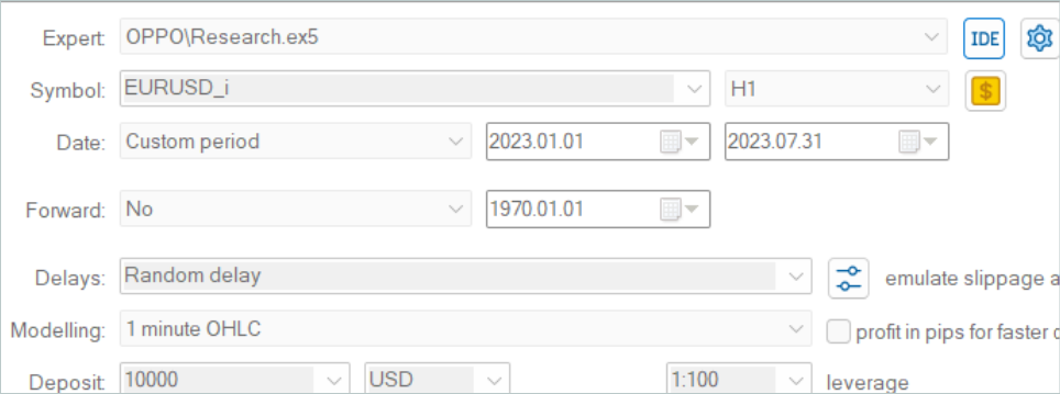
As always, the model is trained on historical data of the EURUSD instrument, H1 time frame for the first 7 months of 2023. The trained model was tested using historical data from August 2023.
Due to changes in the trajectory saving structure in this work, we cannot use example trajectories collected for previous works. Therefore, completely new trajectories were collected into the training dataset.
Here I must admit that collecting 500 trajectories from new models initialized with random weights took 3 days of continuous work on my laptop. This turned out to be quite unexpected.
After collecting the training dataset, I launched parallel training of the models, which was made possible by dividing the training process into 2 independent Expert Advisors.
As always, the learning process was not complete without iterative selection of the training dataset, taking into account model updates. As you will see, the learning process is quite steady and directed. Even if the training dataset has losing passes, the method finds it possible to improve the policy.
According to my personal observation, to build a profitable strategy for the Agent's behavior, the training dataset must have positive passes. The presence of such passes is achieved only by exploring the environment while collecting additional trajectories. It is also possible to use expert trajectories or copy signal transactions, as we have seen in the previous article. And the addition of profitable passes significantly speeds up the model training process.
During the training process, we obtained a model capable of generating profit on both the training and test samples. The model performance results on the test time interval are shown below.


As you can see in the screenshots presented, the balance line has both sharp rises and falls. The balance graph can hardly be called stable, but the general upward trend is preserved. Based on the results of the test month, we made a profit.
During the testing period, the EA executed 180 trades in total. Almost 49% of them were closed with a profit. We can call it parity of profitable and losing trades. However, since the average profitable deal exceeds the average losing one by 30%, we have an overall increase in the balance. The profit factor in this test historical period was 1.25.
Conclusion
In this article, we introduced another rather interesting model training method: Offline Preference-guided Policy Optimization (OPPO). The main feature of this method is the elimination of the reward function from the model training process. Which significantly expands the scope of its use. Because sometimes it can be quite difficult to formulate and specify a certain learning goal. It becomes even more difficult to assess the impact of each individual action on the final outcome, especially in the case of sparse response from the environment. Or when such a response arrives with some delay. Instead, the presented OPPO method evaluates the entire trajectory as a single whole resulting from a single policy. Thus, we evaluate not the Agent's actions, but its policy in a specific environment. And we make decisions to inherit this policy or, on the contrary, to move in the opposite direction to find a more optimal solution.
In the practical part of this article, we implemented the OPPO method using MQL5, although with some deviations from the original method. Nevertheless, we managed to train a policy capable of generating profits both on the training historical period and on the test period beyond the training dataset.
The model training and testing results demonstrate the possibility of using the proposed approaches to build real trading strategies.
However, once again, I would like to remind you that all the programs presented in the article are intended only to demonstrate the technology and are not ready for use in real-world financial trading.
References
Programs used in the article
| # | Name | Type | Description |
|---|---|---|---|
| 1 | Research.mq5 | EA | Example collection EA |
| 2 | StudyAgent.mq5 | EA | Agent training EA |
| 3 | StudyScheduler.mq5 | EA | Preference model training Expert Advisor |
| 4 | Test.mq5 | EA | Model testing EA |
| 5 | Trajectory.mqh | Class library | System state description structure |
| 6 | NeuroNet.mqh | Class library | A library of classes for creating a neural network |
| 7 | NeuroNet.cl | Code Base | OpenCL program code library |
Translated from Russian by MetaQuotes Ltd.
Original article: https://www.mql5.com/ru/articles/13912
Warning: All rights to these materials are reserved by MetaQuotes Ltd. Copying or reprinting of these materials in whole or in part is prohibited.
This article was written by a user of the site and reflects their personal views. MetaQuotes Ltd is not responsible for the accuracy of the information presented, nor for any consequences resulting from the use of the solutions, strategies or recommendations described.

- Free trading apps
- Over 8,000 signals for copying
- Economic news for exploring financial markets
You agree to website policy and terms of use