
Neural networks made easy (Part 63): Unsupervised Pretraining for Decision Transformer (PDT)

Introduction
Decision Transformer is a powerful tool for solving various practical problems. This is largely achieved through the use of Transformer attention methods. Previous experiments have shown that using the Transformer architecture also requires long and thorough model training. This, in turn, requires the preparation of labeled training data. When solving practical problems, it is sometimes quite difficult to get rewards, while labeled data does not scale well to expand the training set. If we do not use rewards during pre-training, the model can acquire general behavioral patterns that can be easily adapted for use in various tasks later.
In this article, I invite you to get acquainted with the RL pretraining method called Pretrained Decision Transformer (PDT), which was presented in the article "Future-conditioned Unsupervised Pretraining for Decision Transformer" in May 2023. This method provides DT with the ability to train on data without reward labels and using suboptimal data. In particular, the authors of the method consider a pre-training scenario in which the model is first trained offline on previously collected trajectories without reward labels, and then fine-tuned to the target task through online interaction.
For effective pre-training, the model must be able to extract multifaceted and universal learning signals without the use of rewards. During pretraining, the model must quickly adapt to the reward task by determining which learning signals can be associated with rewards.
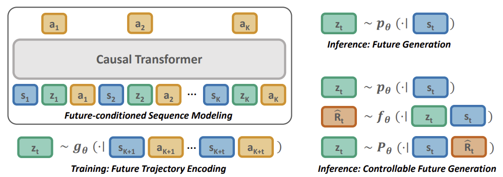
PDT jointly learns an embedding space of future trajectory as well as a future prior conditioned only on past information.. By conditioning action prediction on the target future embedding, PDT is endowed with the ability to "reason over the future". This ability is naturally task-independent and can be generalized to different task specifications.
To achieve efficient online fine-tuning in downstream tasks, you can easily adapt the framework to new conditions by associating each future embedding to its return, which is realized by training a reward prediction network for each future embedding.
I suggest moving on to the next section of our article and considering in detail the Pretrained Decision Transformer method.
1. Pretrained Decision Transformer Method (PDT)
The PDT method is based on the principles of DT. It also predicts the Agent's actions after analyzing the sequence of visited states and completed actions. At the same time, PDT introduces additions to the DT algorithm, allowing preliminary model training on unlabeled data, i. e. without analyzing the return. This seems impossible, because the 'Return-To-Go' (future reward) is one of the members of the sequence analyzed by the model and serves as a kind of compass for the model orientation in space.
The authors of the PDT method proposed replacing RTG with some latent state vector Z. This idea is not new, but the authors gave a rather interesting interpretation of it. In the process of preliminary training on unlabeled data, we will actually train 3 models:
- Actor, which is a classic DT with action prediction based on the analysis of the previous trajectory;
- Target prediction model P(•|St) — predicts DT targets (latent state Z) based on the analysis of the current state;
- Model of the future encoder G(•|τt+1:t+k) — "looks into the future" and embeds it into the latent state Z.
Note that the last 2 models analyze different data, but both return the latent vector Z. This builds a kind of autoencoder between current and future states. Its latent state is used as a target designation for the DT (Actor).
However, model training is different from autoencoder training. First, we train the future encoder and the Actor by building dependencies between the future trajectory and the actions taken. We allow PDT to look into the future for some planning horizon. We compress information about the subsequent trajectory into a latent state. In this way, we allow the model to make a decision based on the available information about the future. We expect during preliminary training to create an Actor policy with a wide range of behavioral skills, unlimited by environmental rewards.
Then we train a target prediction model that looks for dependencies between the current state and the learned embedding of the future trajectory.
This approach allows us to separate rewards from target outcomes, opening up opportunities for large-scale continuous prelearning. At the same time, it reduces the problem of inconsistent behavior when the Agent's behavior significantly deviates from the desired target.
Although the use of the target prediction model P(Z|St) is useful for sampling future latent variables and generating behaviors that mimic the distribution of the training dataset, it does not encode any task-specific data. Therefore it is necessary to send P(Z|St) to a dataset of future embeddings that lead to high future rewards during downstream learning.
This leads to the creation of expert behaviors for the DT, conditioned to maximize returns. Unlike controlling the return-maximizing policy by assigning a scalar target reward, we need to adjust the distribution of the target prediction model P(Z|St). Since this distribution is unknown, we use an additional reward prediction model F(•|Z, St) to predict the optimal trajectory. The reward prediction model learns along with all others during the downstream training process.
Similar to pretraining, we use a future encoder to obtain the latent state, which allows gradients to propagate back, adjusting the encoding of reward data in the latent representation. This allows the solution of the specifics of the task during the downstream learning process.
Below is a visualization of the Pretrained Decision Transformer method from the original article.
2. Implementation using MQL5
Now that we have considered the theoretical aspects of the Pretrained Decision Transformer method, we can move on to the practical part of our article and discuss the implementation of the method in MQL5. In this article, we will focus on the training dataset collecting EA. In previous articles, we considered several options for constructing algorithms from the Decision Transformer family. They all contain a similar experience replay buffer. We will use the for the initial collection of the training dataset. In my work, I will use the experience replay buffer collected in the previous article. We collected it by random sampling of actions without reference to a specific model (implemented for the Go-Explore method).
2.1. Model architecture
Since we already have a set of training data, we move on to the next stage which is the Unsupervised Pretraining. As mentioned above, at this stage we will train 3 models. Let's begin our work with a description of the model architecture, which is collected in the CreateDescriptions method.
bool CreateDescriptions(CArrayObj *agent, CArrayObj *planner, CArrayObj *future_embedding)
  {
//---
   CLayerDescription *descr;
In the parameters, the method receives pointers to 3 dynamic arrays, into which we will add the architecture descriptions of the model's neural layers.
In the body of the method, we declare a local variable to write a pointer to an object describing one neural layer. In this variable, it we will "keep" a pointer to the object with which we are working in a separate block.
First, we will describe the architecture of our Agent. In this case, it is Decision Transformer. It takes as input a step-by-step description of the trajectory and accumulates embeddings of the entire sequence in the results buffer of the Embedding layer. But unlike previous works, during the backpropagation pass, we have to propagate the error gradient to the future encoder model. To do this, we will use a little trick. We will divide the entire source data array into 2 streams. The main amount of data will be passed to the model as usual through the buffer of the source data layer. The embedding of the future will be passed as a second stream to be combined in the concatenation layer. As for the unprocessed source data that we feed into the source data layer buffer, we will normalize it using a batch normalization layer. The embedding of the future is the result of the model's operation and can be used without normalization.
//---
   if(!agent)
     {
      agent = new CArrayObj();
      if(!agent)
         return false;
     }
//--- Agent
   agent.Clear();
//--- Input layer
   if(!(descr = new CLayerDescription()))
      return false;
   descr.type = defNeuronBaseOCL;
   int prev_count = descr.count = (BarDescr * NBarInPattern + AccountDescr + TimeDescription + NActions);
   descr.activation = None;
   descr.optimization = ADAM;
   if(!agent.Add(descr))
     {
      delete descr;
      return false;
     }
//--- layer 1
   if(!(descr = new CLayerDescription()))
      return false;
   descr.type = defNeuronBatchNormOCL;
   descr.count = prev_count;
   descr.batch = 1000;
   descr.activation = None;
   descr.optimization = ADAM;
   if(!agent.Add(descr))
     {
      delete descr;
      return false;
     }
//--- layer 2
   if(!(descr = new CLayerDescription()))
      return false;
   descr.type = defNeuronConcatenate;
   descr.count = prev_count + EmbeddingSize;
   descr.step = EmbeddingSize;
   descr.optimization = ADAM;
   descr.activation = None;
   if(!agent.Add(descr))
     {
      delete descr;
      return false;
     }
The data combined into a single stream is fed to the neural layer of the presented information embedding.
//--- layer 3
   if(!(descr = new CLayerDescription()))
      return false;
   descr.type = defNeuronEmbeddingOCL;
   prev_count = descr.count = HistoryBars;
     {
      int temp[] = {BarDescr * NBarInPattern, AccountDescr, TimeDescription, NActions, EmbeddingSize};
      ArrayCopy(descr.windows, temp);
     }
   int prev_wout = descr.window_out = EmbeddingSize;
   if(!agent.Add(descr))
     {
      delete descr;
      return false;
     }
Then the data is passed to the Transformer block. I used a 4-layer 'cake' with 16 Self-Attention heads.
//--- layer 4
   if(!(descr = new CLayerDescription()))
      return false;
   descr.type = defNeuronMLMHSparseAttentionOCL;
   prev_count = descr.count = prev_count * 5;
   descr.window = EmbeddingSize;
   descr.step = 16;
   descr.window_out = 64;
   descr.layers = 4;
   descr.probability = Sparse;
   descr.optimization = ADAM;
   if(!agent.Add(descr))
     {
      delete descr;
      return false;
     }
After the Transformer block, I used 2 convolutional layers to identify stable patterns.
//--- layer 5
   if(!(descr = new CLayerDescription()))
      return false;
   descr.type = defNeuronConvOCL;
   descr.count = prev_count;
   descr.window = EmbeddingSize;
   descr.step = EmbeddingSize;
   descr.window_out = EmbeddingSize;
   descr.optimization = ADAM;
   descr.activation = LReLU;
   if(!agent.Add(descr))
     {
      delete descr;
      return false;
     }
//--- layer 6
   if(!(descr = new CLayerDescription()))
      return false;
   descr.type = defNeuronConvOCL;
   descr.count = prev_count;
   descr.window = EmbeddingSize;
   descr.step = EmbeddingSize;
   descr.window_out = 16;
   descr.optimization = ADAM;
   descr.activation = LReLU;
   if(!agent.Add(descr))
     {
      delete descr;
      return false;
     }
They are followed by 3 fully connected layers of the decision block.
//--- layer 7
   if(!(descr = new CLayerDescription()))
      return false;
   descr.type = defNeuronBaseOCL;
   descr.count = LatentCount;
   descr.optimization = ADAM;
   descr.activation = LReLU;
   if(!agent.Add(descr))
     {
      delete descr;
      return false;
     }
//--- layer 8
   if(!(descr = new CLayerDescription()))
      return false;
   descr.type = defNeuronBaseOCL;
   prev_count = descr.count = LatentCount;
   descr.activation = LReLU;
   descr.optimization = ADAM;
   if(!agent.Add(descr))
     {
      delete descr;
      return false;
     }
//--- layer 9
   if(!(descr = new CLayerDescription()))
      return false;
   descr.type = defNeuronBaseOCL;
   descr.count = LatentCount;
   descr.activation = LReLU;
   descr.optimization = ADAM;
   if(!agent.Add(descr))
     {
      delete descr;
      return false;
     }
//--- layer 10
   if(!(descr = new CLayerDescription()))
      return false;
   descr.type = defNeuronBaseOCL;
   descr.count = NActions;
   descr.activation = SIGMOID;
   descr.optimization = ADAM;
   if(!agent.Add(descr))
     {
      delete descr;
      return false;
     }
At the output of the model, we have is a fully connected layer with the number of elements equal to the Agent's action space.
Next we will create a description of the target prediction model P(Z|St). Using the terminology of hierarchical models, we can call it the Planner. Their functionality is structurally very similar, although the approaches to training models are radically different.
As an input to the model's source data layer, we feed a description of only historical data and indicator values for one pattern. In our case, this is data from only 1 bar.
I agree that this is too little information to analyze the market situation and predict future states and actions. Especially if we talk about predictions a few steps forward. But let's look at the situation differently. During operation, we feed the generated future prediction in the form of embedding as an input to our Actor. Its internal layers store data to a given depth of history. In this context, it is more important for us to pay attention to the changes that have occurred and adjust the Actor's behavior. Analyzing a deeper history when creating the future embedding can "blur" local changes. However, this is my subjective opinion and is not a requirement of the Pretrained Decision Transformer algorithm.
   if(!planner)
     {
      planner = new CArrayObj();
      if(!planner)
         return false;
     }
//--- Planner
   planner.Clear();
//--- Input layer
   if(!(descr = new CLayerDescription()))
      return false;
   descr.type = defNeuronBaseOCL;
   prev_count = descr.count = BarDescr * NBarInPattern;
   descr.activation = None;
   descr.optimization = ADAM;
   if(!planner.Add(descr))
     {
      delete descr;
      return false;
     }
The resulting raw data is passed through a batch normalization layer to convert it into a comparable form.
//--- layer 1
   if(!(descr = new CLayerDescription()))
      return false;
   descr.type = defNeuronBatchNormOCL;
   descr.count = prev_count;
   descr.batch = 1000;
   descr.activation = None;
   descr.optimization = ADAM;
   if(!planner.Add(descr))
     {
      delete descr;
      return false;
     }
Next, I decided not to complicate the model and used a decision-making block of 3 fully connected layers.
//--- layer 2
   if(!(descr = new CLayerDescription()))
      return false;
   descr.type = defNeuronBaseOCL;
   descr.count = LatentCount;
   descr.optimization = ADAM;
   descr.activation = LReLU;
   if(!planner.Add(descr))
     {
      delete descr;
      return false;
     }
//--- layer 3
   if(!(descr = new CLayerDescription()))
      return false;
   descr.type = defNeuronBaseOCL;
   prev_count = descr.count = LatentCount;
   descr.activation = LReLU;
   descr.optimization = ADAM;
   if(!planner.Add(descr))
     {
      delete descr;
      return false;
     }
//--- layer 4
   if(!(descr = new CLayerDescription()))
      return false;
   descr.type = defNeuronBaseOCL;
   prev_count = descr.count = LatentCount;
   descr.activation = LReLU;
   descr.optimization = ADAM;
   if(!planner.Add(descr))
     {
      delete descr;
      return false;
     }
At the output of the model, we reduce the vector size down to the embedding size and normalize the results using the SoftMax functions.
//--- layer 5
   if(!(descr = new CLayerDescription()))
      return false;
   descr.type = defNeuronBaseOCL;
   prev_count = descr.count = EmbeddingSize;
   descr.activation = None;
   descr.optimization = ADAM;
   if(!planner.Add(descr))
     {
      delete descr;
      return false;
     }
//--- layer 6
   if(!(descr = new CLayerDescription()))
      return false;
   descr.type = defNeuronSoftMaxOCL;
   descr.count = EmbeddingSize;
   descr.activation = None;
   descr.optimization = ADAM;
   if(!planner.Add(descr))
     {
      delete descr;
      return false;
     }
We have already described the architectural solution of 2 models. And all we have to do is add a description of the future encoder. Although the output of the model is basically intended to match the output of the previous model, this will only be noticeable in the last layers of the model. The encoder architecture is a little more complicated. First of all, in the future embedding we enable planning to some depth. This means that we feed information about several subsequent candles into the source data layer.
Note that in the data about the future, I included only data on the symbol price movement and indicator readings. I did not include information about the account state and subsequent actions of the Agent. The Agent's actions are determined by its policy. I wanted to focus on understanding processes in the environment. While the account state to some extent already contains information about the reward received from the environment, which somewhat contradicts the principle of unlabeled data.
//--- Future Embedding
   if(!future_embedding)
     {
      future_embedding = new CArrayObj();
      if(!future_embedding)
         return false;
     }
//---
   future_embedding.Clear();
//--- Input layer
   if(!(descr = new CLayerDescription()))
      return false;
   descr.type = defNeuronBaseOCL;
   prev_count = descr.count = BarDescr * NBarInPattern * ValueBars;
   descr.activation = None;
   descr.optimization = ADAM;
   if(!future_embedding.Add(descr))
     {
      delete descr;
      return false;
     }
//--- layer 1
   if(!(descr = new CLayerDescription()))
      return false;
   descr.type = defNeuronBatchNormOCL;
   descr.count = prev_count;
   descr.batch = 1000;
   descr.activation = None;
   descr.optimization = ADAM;
   if(!future_embedding.Add(descr))
     {
      delete descr;
      return false;
     }
As before, we pass the raw unprocessed data through a batch normalization layer to convert it to a comparable form.
Next I used a 4-layer Transformer block and 16 Self-Attention heads. In this case, the attention block analyzes the dependencies between individual bars in an attempt to identify the main trends on the planning horizon and filter out the noise component.
According to the PDT method logic, it is the embedding of the future state that should indicate to the Actor the skill being used and the direction of further actions. Therefore, the result of the encoder operation should be as informative and accurate as possible.
//--- layer 2
   if(!(descr = new CLayerDescription()))
      return false;
   descr.type = defNeuronMLMHSparseAttentionOCL;
   prev_count = descr.count = ValueBars;
   descr.window = BarDescr * NBarInPattern;
   descr.step = 16;
   descr.window_out = 64;
   descr.layers = 4;
   descr.probability = Sparse;
   descr.optimization = ADAM;
   if(!future_embedding.Add(descr))
     {
      delete descr;
      return false;
     }
The attention layers are followed by fully connected layers of the decision block.
//--- layer 3
   if(!(descr = new CLayerDescription()))
      return false;
   descr.type = defNeuronBaseOCL;
   descr.count = LatentCount;
   descr.optimization = ADAM;
   descr.activation = LReLU;
   if(!future_embedding.Add(descr))
     {
      delete descr;
      return false;
     }
//--- layer 4
   if(!(descr = new CLayerDescription()))
      return false;
   descr.type = defNeuronBaseOCL;
   prev_count = descr.count = LatentCount;
   descr.activation = LReLU;
   descr.optimization = ADAM;
   if(!future_embedding.Add(descr))
     {
      delete descr;
      return false;
     }
At the model output, we use a fully connected layer with SoftMax normalization, as was done above in the future forecasting model.
//--- layer 5
   if(!(descr = new CLayerDescription()))
      return false;
   descr.type = defNeuronBaseOCL;
   descr.count = EmbeddingSize;
   descr.activation = None;
   descr.optimization = ADAM;
   if(!future_embedding.Add(descr))
     {
      delete descr;
      return false;
     }
//--- layer 6
   if(!(descr = new CLayerDescription()))
      return false;
   descr.type = defNeuronSoftMaxOCL;
   descr.count = EmbeddingSize;
   descr.activation = None;
   descr.optimization = ADAM;
   if(!future_embedding.Add(descr))
     {
      delete descr;
      return false;
     }
//---
   return true;
  }
This concludes the description of the model architecture for the pretraining Expert Advisor. But before moving on to working on the Expert Advisor, I would like to complete the work on describing the architecture of the models. I would like to remind you that at the stage of fine-tuning using the PDT method, it is possible to add another model which is reward prediction. Since it is added at a subsequent stage of training, I decided to include a description of its architecture in a separate CreateValueDescriptions method.
According to the PDT methodology, this model must estimate future trends encoded in the latent state and the current state. Based on the results of the analysis, it is necessary to predict rewards from the environment.
The purpose of the downstream training process is to include information about the probable reward in the future embedding. Therefore, as in the pretraining stage, we need to pass the reward prediction error gradient to the future encoder model. Here we will use the approach tested above to separate information flows. One of the initial data streams will be the current state. The second one will be the future embedding.
The second question that we now have to solve is what is included in understanding the current state at this stage. Of course, at the fine-tuning stage we use labeled data from the training dataset and could include the entire amount of available data. But a large volume of input data greatly complicates the model and increases the cost of the model processing. What is the effectiveness of using such an amount of data at the current stage?
To predict subsequent states, we need to analyze the previous states of the environment. But we already have information about future states in the form of embedding.
The analysis of the Agent's previous actions can indicate the policy being used. But we need to provide information to the Agent to make a decision about the need to change the skill and behavior policy used.
Information about the current account status can be useful. The presence of free margin will indicate that additional positions can be opened if the trend is favorable. Or, if the trends are expected to change, and we have to close previously open positions and lock in floating profits and losses. In addition, we should remember about penalties for the lack of open positions, which will also affect the reward.
Therefore, we feed the current description of the account status and open positions into the source data layer.
bool CreateValueDescriptions(CArrayObj *value)
  {
//---
   CLayerDescription *descr;
//---
   if(!value)
     {
      value = new CArrayObj();
      if(!value)
         return false;
     }
//--- Value
   value.Clear();
//--- Input layer
   if(!(descr = new CLayerDescription()))
      return false;
   descr.type = defNeuronBaseOCL;
   int prev_count = descr.count = AccountDescr;
   descr.activation = None;
   descr.optimization = ADAM;
   if(!value.Add(descr))
     {
      delete descr;
      return false;
     }
The output is passed through a batch normalization layer.
//--- layer 1
   if(!(descr = new CLayerDescription()))
      return false;
   descr.type = defNeuronBatchNormOCL;
   descr.count = prev_count;
   descr.batch = 1000;
   descr.activation = None;
   descr.optimization = ADAM;
   if(!value.Add(descr))
     {
      delete descr;
      return false;
     }
Next, we combine the 2 data streams in the concatenation layer.
//--- layer 2
   if(!(descr = new CLayerDescription()))
      return false;
   descr.type = defNeuronConcatenate;
   descr.count = LatentCount;
   descr.step = EmbeddingSize;
   descr.optimization = ADAM;
   descr.activation = SIGMOID;
   if(!value.Add(descr))
     {
      delete descr;
      return false;
     }
Then the data is passed to the decision-making block from the fully connected layers.
//--- layer 3
   if(!(descr = new CLayerDescription()))
      return false;
   descr.type = defNeuronBaseOCL;
   descr.count = LatentCount;
   descr.optimization = ADAM;
   descr.activation = LReLU;
   if(!value.Add(descr))
     {
      delete descr;
      return false;
     }
//--- layer 4
   if(!(descr = new CLayerDescription()))
      return false;
   descr.type = defNeuronBaseOCL;
   prev_count = descr.count = LatentCount;
   descr.activation = LReLU;
   descr.optimization = ADAM;
   if(!value.Add(descr))
     {
      delete descr;
      return false;
     }
//--- layer 5
   if(!(descr = new CLayerDescription()))
      return false;
   descr.type = defNeuronBaseOCL;
   descr.count = NRewards;
   descr.activation = None;
   descr.optimization = ADAM;
   if(!value.Add(descr))
     {
      delete descr;
      return false;
     }
//---
   return true;
  }
At the model output, we get a vector of expected rewards.
2.2. Pretraining Expert Advisor
After creating the architecture of the models used, let's proceed to implement the PDT method algorithm. We start with the pretraining Expert Advisor "...\PDT\Pretrain.mq5". As mentioned above, this EA performed preliminary training of 3 models: Actor, Planner and Future Encoder.
CNet                 Agent;
CNet                 Planner;
CNet                 FutureEmbedding;
In the EA initialization method, we first load the training dataset.
//+------------------------------------------------------------------+
//| Expert initialization function                                   |
//+------------------------------------------------------------------+
int OnInit()
  {
//---
   ResetLastError();
   if(!LoadTotalBase())
     {
      PrintFormat("Error of load study data: %d", GetLastError());
      return INIT_FAILED;
     }
Make an attempt to load pretrained models and, if necessary, to initialize new models according to the architecture described above.
//--- load models
   float temp;
   if(!Agent.Load(FileName + "Act.nnw", temp, temp, temp, dtStudied, true) ||
      !Planner.Load(FileName + "Pln.nnw", temp, temp, temp, dtStudied, true) ||
      !FutureEmbedding.Load(FileName + "FEm.nnw", temp, temp, temp, dtStudied, true))
     {
      CArrayObj *agent = new CArrayObj();
      CArrayObj *planner = new CArrayObj();
      CArrayObj *future_embedding = new CArrayObj();
      if(!CreateDescriptions(agent, planner, future_embedding))
        {
         delete agent;
         delete planner;
         delete future_embedding;
         return INIT_FAILED;
        }
      if(!Agent.Create(agent) || !Planner.Create(planner) ||
         !FutureEmbedding.Create(future_embedding))
        {
         delete agent;
         delete planner;
         delete future_embedding;
         return INIT_FAILED;
        }
      delete agent;
      delete planner;
      delete future_embedding;
      //---
     }
Then we transfer all models into one OpenCL context.
//---
   COpenCL *opcl = Agent.GetOpenCL();
   Planner.SetOpenCL(opcl);
   FutureEmbedding.SetOpenCL(opcl);
Here we perform the minimal required control over the model architecture.
   Agent.getResults(Result);
   if(Result.Total() != NActions)
     {
      PrintFormat("The scope of the worker does not match the actions count (%d <> %d)", NActions, Result.Total());
      return INIT_FAILED;
     }
Initialize the launch of the preliminary training process, which is implemented in the Train method.
//---
   if(!EventChartCustom(ChartID(), 1, 0, 0, "Init"))
     {
      PrintFormat("Error of create study event: %d", GetLastError());
      return INIT_FAILED;
     }
//---
   return(INIT_SUCCEEDED);
  }
In the EA deinitializaiton method, we must save the trained models.
//+------------------------------------------------------------------+
//| Expert deinitialization function                                 |
//+------------------------------------------------------------------+
void OnDeinit(const int reason)
  {
//---
   Agent.Save(FileName + "Act.nnw", 0, 0, 0, TimeCurrent(), true);
   Planner.Save(FileName + "Pln.nnw", 0, 0, 0, TimeCurrent(), true);
   FutureEmbedding.Save(FileName + "FEm.nnw", 0, 0, 0, TimeCurrent(), true);
   delete Result;
  }
The model training process is implemented in the Train method. In the method body, we first determine the size of the experience replay buffer.
//+------------------------------------------------------------------+
//| Train function                                                   |
//+------------------------------------------------------------------+
void Train(void)
  {
   int total_tr = ArraySize(Buffer);
   uint ticks = GetTickCount();
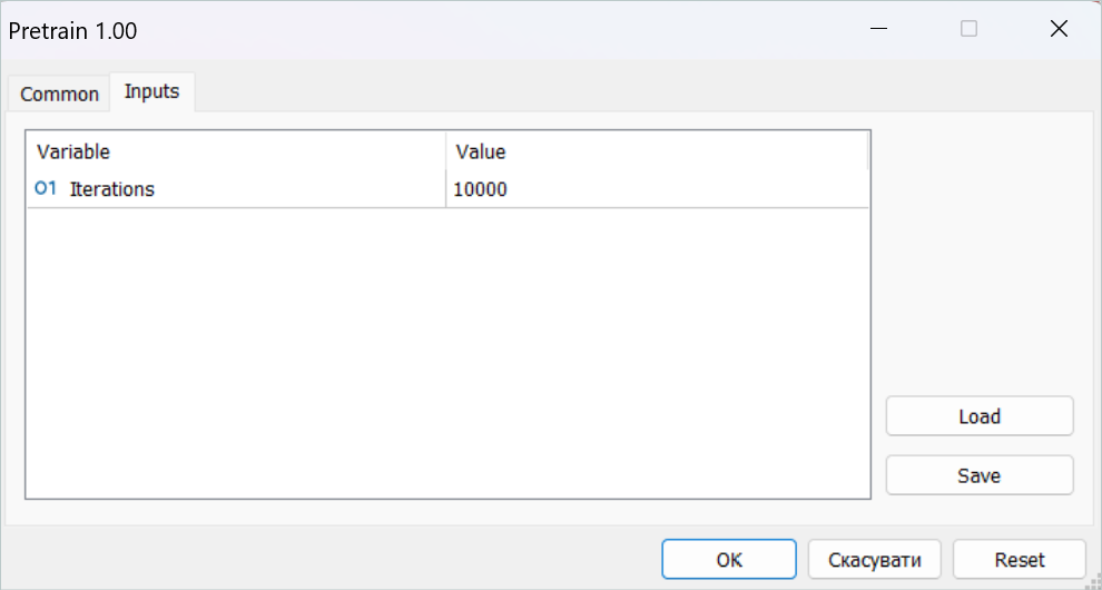
Next, we created a system of nested loops for the model training process. The external loop is limited to the number of training iterations specified in the EA external parameters. In the body of this loop, we first sample a trajectory from the experience replay buffer and a separate environmental state along the selected trajectory to begin the learning process.
   bool StopFlag = false;
   for(int iter = 0; (iter < Iterations && !IsStopped() && !StopFlag); iter ++)
     {
      int tr = (int)((MathRand() / 32767.0) * (total_tr - 1));
      int i = (int)((MathRand() * MathRand() / MathPow(32767, 2)) * MathMax(Buffer[tr].Total - 2 * HistoryBars - ValueBars,
                                                                            MathMin(Buffer[tr].Total, 20 + ValueBars)));
      if(i < 0)
        {
         iter--;
         continue;
        }
After that we run a nested loop to train the DT model sequentially.
      Actions = vector<float>::Zeros(NActions);
      for(int state = i; state < MathMin(Buffer[tr].Total - ValueBars, i + HistoryBars * 3); state++)
        {
         //--- History data
         State.AssignArray(Buffer[tr].States[state].state);
         if(!Planner.feedForward(GetPointer(State), 1, false))
           {
            PrintFormat("%s -> %d", __FUNCTION__, __LINE__);
            StopFlag = true;
            break;
           }
In the body of the loop, we write historical price movement data and indicator readings to the source data buffer. Note that this data is actually sufficient to run a feed-forward pass of the Planner model. This operation will run first. After that we continue filling the source data buffer for our Actor. Add the account state.
         //--- Account description
         float PrevBalance = (state == 0 ? Buffer[tr].States[state].account[0] : Buffer[tr].States[state - 1].account[0]);
         float PrevEquity = (state == 0 ? Buffer[tr].States[state].account[1] : Buffer[tr].States[state - 1].account[1]);
         State.Add((Buffer[tr].States[state].account[0] - PrevBalance) / PrevBalance);
         State.Add(Buffer[tr].States[state].account[1] / PrevBalance);
         State.Add((Buffer[tr].States[state].account[1] - PrevEquity) / PrevEquity);
         State.Add(Buffer[tr].States[state].account[2]);
         State.Add(Buffer[tr].States[state].account[3]);
         State.Add(Buffer[tr].States[state].account[4] / PrevBalance);
         State.Add(Buffer[tr].States[state].account[5] / PrevBalance);
         State.Add(Buffer[tr].States[state].account[6] / PrevBalance);
Add the timestamp and last actions of the Agent.
         //--- Time label
         double x = (double)Buffer[tr].States[state].account[7] / (double)(D'2024.01.01' - D'2023.01.01');
         State.Add((float)MathSin(2.0 * M_PI * x));
         x = (double)Buffer[tr].States[state].account[7] / (double)PeriodSeconds(PERIOD_MN1);
         State.Add((float)MathCos(2.0 * M_PI * x));
         x = (double)Buffer[tr].States[state].account[7] / (double)PeriodSeconds(PERIOD_W1);
         State.Add((float)MathSin(2.0 * M_PI * x));
         x = (double)Buffer[tr].States[state].account[7] / (double)PeriodSeconds(PERIOD_D1);
         State.Add((float)MathSin(2.0 * M_PI * x));
         //--- Prev action
         State.AddArray(Actions);
Now, to perform a feed-forward pass of the Actor, we only need the embedding of the future. Well, we have a buffer of Planner results, but at this stage the result of the untrained model is not conditioned by anything. According to the PDT algorithm, we need to load informatio about subsequent states and generate an embedding of the received data.
         //--- Target
         Result.AssignArray(Buffer[tr].States[state + 1].state);
         for(int s = 1; s < ValueBars; s++)
            Result.AddArray(Buffer[tr].States[state + 1].state);
         if(!FutureEmbedding.feedForward(Result, 1, false))
           {
            PrintFormat("%s -> %d", __FUNCTION__, __LINE__);
            StopFlag = true;
            break;
           }
The encoder operation result is input into the 2nd Actor model. Next we call its direct pass.
         FutureEmbedding.getResults(Result);
         //--- Policy Feed Forward
         if(!Agent.feedForward(GetPointer(State), 1, false, Result))
           {
            PrintFormat("%s -> %d", __FUNCTION__, __LINE__);
            StopFlag = true;
            break;
           }
After performing the forward pass through all the models used, we proceed to train them. First we call the backpropagation method for the Planner model (forecasting the future). This sequence is related to the readiness of the vector of target results that we just input into the Actor.
         //--- Planner Study
         if(!Planner.backProp(Result, NULL, NULL))
           {
            PrintFormat("%s -> %d", __FUNCTION__, __LINE__);
            StopFlag = true;
            break;
           }
Next, move on to preparing our Actor's target returns. To do this, we use actions from the experience replay buffer that led to known consequences.
         //--- Policy study
         Actions.Assign(Buffer[tr].States[state].action);
         vector<float> result;
         Agent.getResults(result);
         Result.AssignArray(CAGrad(Actions - result) + result);
After preparing the target values, we perform a backpropagation run of the Actor and immediately pass the error gradient through the future encoder model.
         if(!Agent.backProp(Result, GetPointer(FutureEmbedding)) ||
            !FutureEmbedding.backPropGradient((CBufferFloat *)NULL))
           {
            PrintFormat("%s -> %d", __FUNCTION__, __LINE__);
            StopFlag = true;
            break;
           }
After that we only need to inform the user about the progress of the operations and move on to a new iteration.
         //---
         if(GetTickCount() - ticks > 500)
           {
            string str = StringFormat("%-15s %5.2f%% -> Error %15.8f\n", "Agent", iter * 100.0 /
                                                        (double)(Iterations), Agent.getRecentAverageError());
            str += StringFormat("%-15s %5.2f%% -> Error %15.8f\n", "Planner", iter * 100.0 /
                                                        (double)(Iterations), Planner.getRecentAverageError());
            Comment(str);
            ticks = GetTickCount();
           }
        }
     }
When all iterations of the loop system are completed, we clear the chart comments field. Display the training results in the journal and initiate EA termination.
   Comment("");
//---
   PrintFormat("%s -> %d -> %-15s %10.7f", __FUNCTION__, __LINE__, "Agent", Agent.getRecentAverageError());
   PrintFormat("%s -> %d -> %-15s %10.7f", __FUNCTION__, __LINE__, "Planner", Planner.getRecentAverageError());
   ExpertRemove();
//---
  }
All other EA methods have been transferred without changes from training Expert Advisors earlier considered in other articles "...\Study.mq5". So, we will not dwell on them now. You can find the full code of the program in the attachment. We are moving on to the next stage of our work.
2.3. Fine-tuning EA
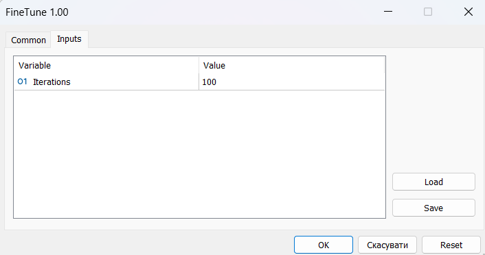
After completing the implementation of the pretraining algorithm, we proceed to work on creating the fine-tuning EA "...\PDT\FineTune.mq5", in which we will build an algorithm for downstream training of models.
The Expert Advisor is approximately 90% the same as the previous one. Therefore, we will not consider all its methods in detail. We will only see the changes made.
As mentioned in the theoretical part of this article, the PDT method at this stage allows the optimization of models to solve the problem. This means that we will use labeled data and environmental rewards to optimize our Agent's policies. Therefore, we add another external reward prediction model to the learning process.
CNet RTG;
Please note that we only add a model, leaving the use of models from the previous Expert Advisor unchanged.
In the fine-tuning Expert Advisor, I left a mechanism for creating new models of the Agent, Planner and Future Encoder if it is impossible to load pretrained models. Thus, users can train models from scratch. At the same time, loading and, if necessary, initialization of a new external reward forecasting model in the Expert Advisor initialization method are arranged in a separate block. When moving from pretraining to fine-tuning, we will have models trained in the previous EA. As for the reward prediction model, we will initialize it with random parameters.
//+------------------------------------------------------------------+
//| Expert initialization function                                   |
//+------------------------------------------------------------------+
int OnInit()
  {
//---
........
........
//---
   if(!RTG.Load(FileName + "RTG.nnw", temp, temp, temp, dtStudied, true))
     {
      CArrayObj *rtg = new CArrayObj();
      if(!CreateValueDescriptions(rtg))
        {
         delete rtg;
         return INIT_FAILED;
        }
      if(!RTG.Create(rtg))
        {
         delete rtg;
         return INIT_FAILED;
        }
      delete rtg;
      //---
     }
//---
   COpenCL *opcl = Agent.GetOpenCL();
   Planner.SetOpenCL(opcl);
   FutureEmbedding.SetOpenCL(opcl);
   RTG.SetOpenCL(opcl);
//---
   RTG.getResults(Result);
   if(Result.Total() != NRewards)
     {
      PrintFormat("The scope of the RTG does not match the rewards count (%d <> %d)", NRewards, Result.Total());
      return INIT_FAILED;
     }
//---
........
........
//---
   return(INIT_SUCCEEDED);
  }
Next, we transfer all models into a single OpenCL context and check if the results layer of the added model matches the dimension of the decomposed reward vector.
Some additions have also been made to the Train model training method. After the Agent's feed-forward pass, we add a call to the reward prediction model's feed-forward pass. As discussed above, for the input of the model, we feed a vector describing the account state and the future embedding.
........
........
         //--- Policy Feed Forward
         if(!Agent.feedForward(GetPointer(State), 1, false, Result))
           {
            PrintFormat("%s -> %d", __FUNCTION__, __LINE__);
            StopFlag = true;
            break;
           }
         //--- Return-To-Go
         Account.AssignArray(Buffer[tr].States[state + 1].account);
         if(!RTG.feedForward(GetPointer(Account), 1, false, Result))
           {
            PrintFormat("%s -> %d", __FUNCTION__, __LINE__);
            StopFlag = true;
            break;
           }
........
........
The model parameters are also updated after the Agent parameters are updated. The model optimization algorithms are almost identical. By calling the model's backpropagation method, we propagate the error gradient to the future encoding model and then update its parameters. The only difference is in the target values. This approach allows us to train the dependence of the Agent's actions and the external reward received on future embedding.
........
........
         //--- Policy study
         Actions.Assign(Buffer[tr].States[state].action);
         vector<float> result;
         Agent.getResults(result);
         Result.AssignArray(CAGrad(Actions - result) + result);
         if(!Agent.backProp(Result, GetPointer(FutureEmbedding)) ||
            !FutureEmbedding.backPropGradient((CBufferFloat *)NULL))
           {
            PrintFormat("%s -> %d", __FUNCTION__, __LINE__);
            StopFlag = true;
            break;
           }
         //--- Return To Go study
         vector<float> target;
         target.Assign(Buffer[tr].States[state + 1].rewards);
         result.Assign(Buffer[tr].States[state + ValueBars].rewards);
         target = target - result * MathPow(DiscFactor, ValueBars);
         Result.AssignArray(target);
         if(!RTG.backProp(Result, GetPointer(FutureEmbedding)) ||
            !FutureEmbedding.backPropGradient((CBufferFloat *)NULL))
           {
            PrintFormat("%s -> %d", __FUNCTION__, __LINE__);
            StopFlag = true;
            break;
           }
........
........
This completes our local changes. The full code of the EA and all programs used in the article are available in the attachment.
2.4. Expert Advisor for testing trained models
After training the models in the Expert Advisors discussed above, we will need to test the performance of the resulting models using historical data that is not included in the training dataset. To implement this functionality, let's create a new Expert Advisor "...\PDT\Test.mq5". Unlike the EAs discussed above, in which models were trained offline, the testing EA interacts online with the environment. This is reflected in the construction of its algorithm.
In the OnInit EA initialization method, we first initialize the objects of the analyzed indicators.
//+------------------------------------------------------------------+
//| Expert initialization function                                   |
//+------------------------------------------------------------------+
int OnInit()
  {
//---
   if(!Symb.Name(_Symbol))
      return INIT_FAILED;
   Symb.Refresh();
//---
   if(!RSI.Create(Symb.Name(), TimeFrame, RSIPeriod, RSIPrice))
      return INIT_FAILED;
//---
   if(!CCI.Create(Symb.Name(), TimeFrame, CCIPeriod, CCIPrice))
      return INIT_FAILED;
//---
   if(!ATR.Create(Symb.Name(), TimeFrame, ATRPeriod))
      return INIT_FAILED;
//---
   if(!MACD.Create(Symb.Name(), TimeFrame, FastPeriod, SlowPeriod, SignalPeriod, MACDPrice))
      return INIT_FAILED;
   if(!RSI.BufferResize(NBarInPattern) || !CCI.BufferResize(NBarInPattern) ||
      !ATR.BufferResize(NBarInPattern) || !MACD.BufferResize(NBarInPattern))
     {
      PrintFormat("%s -> %d", __FUNCTION__, __LINE__);
      return INIT_FAILED;
     }
Creating a trading operations object.
//---
   if(!Trade.SetTypeFillingBySymbol(Symb.Name()))
      return INIT_FAILED;
Loading the trained models. Here we use only 2 models: Actor and Planner. Unlike previous EAs, an error in loading models leads to the interruption of the EA. Because we did not implement online model training in it.
//--- load models
   float temp;
   if(!Agent.Load(FileName + "Act.nnw", temp, temp, temp, dtStudied, true) ||
      !Planner.Load(FileName + "Pln.nnw", temp, temp, temp, dtStudied, true))
     {
      PrintFormat("Can't load pretrained model");
      return INIT_FAILED;
     }
After successfully loading the models, we transfer them into a single OpenCL context and perform the minimum necessary architectural control.
   Planner.SetOpenCL(Agent.GetOpenCL());
   Agent.getResults(Result);
   if(Result.Total() != NActions)
     {
      PrintFormat("The scope of the Actor does not match the actions count (%d <> %d)", NActions, Result.Total());
      return INIT_FAILED;
     }
//---
   Agent.GetLayerOutput(0, Result);
   if(Result.Total() != (BarDescr * NBarInPattern + AccountDescr + TimeDescription + NActions))
     {
      PrintFormat("Input size of Actor doesn't match state description (%d <> %d)", Result.Total(),
                              (NRewards + BarDescr * NBarInPattern + AccountDescr + TimeDescription + NActions));
      return INIT_FAILED;
     }
   Agent.Clear();
At the end of the method, we initialize the variables with initial values.
   AgentResult = vector<float>::Zeros(NActions);
   PrevBalance = AccountInfoDouble(ACCOUNT_BALANCE);
   PrevEquity = AccountInfoDouble(ACCOUNT_EQUITY);
//---
   return(INIT_SUCCEEDED);
  }
The process of interaction with the environment is implemented in the OnTick tick processing method. In the method body, we first check the occurrence of a new bar opening event. This is because all our models analyze closed candlesticks and execute trading operations at the opening of a new bar.
//+------------------------------------------------------------------+
//| Expert tick function                                             |
//+------------------------------------------------------------------+
void OnTick()
  {
//---
   if(!IsNewBar())
      return;
Next, we request from the terminal the necessary data for the analyzed history depth. In this case, by history depth I mean the size of one pattern, which in our case is one bar. The depth of the history analyzed by the Agent is contained in its latent state in the form of embeddings and is not re-processed on each bar.
   int bars = CopyRates(Symb.Name(), TimeFrame, iTime(Symb.Name(), TimeFrame, 1), NBarInPattern, Rates);
   if(!ArraySetAsSeries(Rates, true))
      return;
//---
   RSI.Refresh();
   CCI.Refresh();
   ATR.Refresh();
   MACD.Refresh();
   Symb.Refresh();
   Symb.RefreshRates();
Next, we need to transfer the received data to a buffer to be passed to the model.
//--- History data
   float atr = 0;
   for(int b = 0; b < NBarInPattern; b++)
     {
      float open = (float)Rates[b].open;
      float rsi = (float)RSI.Main(b);
      float cci = (float)CCI.Main(b);
      atr = (float)ATR.Main(b);
      float macd = (float)MACD.Main(b);
      float sign = (float)MACD.Signal(b);
      if(rsi == EMPTY_VALUE || cci == EMPTY_VALUE || atr == EMPTY_VALUE || macd == EMPTY_VALUE || sign == EMPTY_VALUE)
         continue;
      //---
      int shift = b * BarDescr;
      sState.state[shift] = (float)(Rates[b].close - open);
      sState.state[shift + 1] = (float)(Rates[b].high - open);
      sState.state[shift + 2] = (float)(Rates[b].low - open);
      sState.state[shift + 3] = (float)(Rates[b].tick_volume / 1000.0f);
      sState.state[shift + 4] = rsi;
      sState.state[shift + 5] = cci;
      sState.state[shift + 6] = atr;
      sState.state[shift + 7] = macd;
      sState.state[shift + 8] = sign;
     }
   bState.AssignArray(sState.state);
The received historical data is enough to run a feed-forward pass of the Planner.
   if(!Planner.feedForward(GetPointer(bState), 1, false))
      return;
However, for the Agent to function fully, we require additional data. First, we add to the buffer information about the account state, which we first request from the terminal.
//--- Account description
   sState.account[0] = (float)AccountInfoDouble(ACCOUNT_BALANCE);
   sState.account[1] = (float)AccountInfoDouble(ACCOUNT_EQUITY);
//---
   double buy_value = 0, sell_value = 0, buy_profit = 0, sell_profit = 0;
   double position_discount = 0;
   double multiplyer = 1.0 / (60.0 * 60.0 * 10.0);
   int total = PositionsTotal();
   datetime current = TimeCurrent();
   for(int i = 0; i < total; i++)
     {
      if(PositionGetSymbol(i) != Symb.Name())
         continue;
      double profit = PositionGetDouble(POSITION_PROFIT);
      switch((int)PositionGetInteger(POSITION_TYPE))
        {
         case POSITION_TYPE_BUY:
            buy_value += PositionGetDouble(POSITION_VOLUME);
            buy_profit += profit;
            break;
         case POSITION_TYPE_SELL:
            sell_value += PositionGetDouble(POSITION_VOLUME);
            sell_profit += profit;
            break;
        }
      position_discount += profit - (current - PositionGetInteger(POSITION_TIME)) * multiplyer * MathAbs(profit);
     }
   sState.account[2] = (float)buy_value;
   sState.account[3] = (float)sell_value;
   sState.account[4] = (float)buy_profit;
   sState.account[5] = (float)sell_profit;
   sState.account[6] = (float)position_discount;
   sState.account[7] = (float)Rates[0].time;
//---
   bState.Add((float)((sState.account[0] - PrevBalance) / PrevBalance));
   bState.Add((float)(sState.account[1] / PrevBalance));
   bState.Add((float)((sState.account[1] - PrevEquity) / PrevEquity));
   bState.Add(sState.account[2]);
   bState.Add(sState.account[3]);
   bState.Add((float)(sState.account[4] / PrevBalance));
   bState.Add((float)(sState.account[5] / PrevBalance));
   bState.Add((float)(sState.account[6] / PrevBalance));
Next we add a timestamp and the last actions of the Agent.
//--- Time label
   double x = (double)Rates[0].time / (double)(D'2024.01.01' - D'2023.01.01');
   bState.Add((float)MathSin(2.0 * M_PI * x));
   x = (double)Rates[0].time / (double)PeriodSeconds(PERIOD_MN1);
   bState.Add((float)MathCos(2.0 * M_PI * x));
   x = (double)Rates[0].time / (double)PeriodSeconds(PERIOD_W1);
   bState.Add((float)MathSin(2.0 * M_PI * x));
   x = (double)Rates[0].time / (double)PeriodSeconds(PERIOD_D1);
   bState.Add((float)MathSin(2.0 * M_PI * x));
//--- Prev action
   bState.AddArray(AgentResult);
In a separate buffer, we receive the results of the previously performed feed-forward pass of the Planner and call the feed-forward method of the Agent.
//--- Return to go
   Planner.getResults(Result);
//---
   if(!Agent.feedForward(GetPointer(bState), 1, false, Result))
      return;
Then we update the variables necessary for operations on the next bar.
//---
   PrevBalance = sState.account[0];
   PrevEquity = sState.account[1];
The first stage of the initial data analysis is completed. Let's move on to the stage of interaction with the environment. Here we receive the results of the Agent's feed-forward pass and decrypt them into a vector of upcoming operations. As usual, we exclude overlapping volumes and leave the difference in the direction of the more likely movement.
   vector<float> temp;
   Agent.getResults(temp);
//---
   double min_lot = Symb.LotsMin();
   double step_lot = Symb.LotsStep();
   double stops = MathMax(Symb.StopsLevel(), 1) * Symb.Point();
   if(temp[0] >= temp[3])
     {
      temp[0] -= temp[3];
      temp[3] = 0;
     }
   else
     {
      temp[3] -= temp[0];
      temp[0] = 0;
     }
   float delta = MathAbs(AgentResult - temp).Sum();
   AgentResult = temp;
Then we adjust our position in the market according to the forecast values. First we adjust our long position.
//--- buy control
   if(temp[0] < min_lot || (temp[1] * MaxTP * Symb.Point()) <= stops || (temp[2] * MaxSL * Symb.Point()) <= stops)
     {
      if(buy_value > 0)
         CloseByDirection(POSITION_TYPE_BUY);
     }
   else
     {
      double buy_lot = min_lot + MathRound((double)(temp[0] - min_lot) / step_lot) * step_lot;
      double buy_tp = Symb.NormalizePrice(Symb.Ask() + temp[1] * MaxTP * Symb.Point());
      double buy_sl = Symb.NormalizePrice(Symb.Ask() - temp[2] * MaxSL * Symb.Point());
      if(buy_value > 0)
         TrailPosition(POSITION_TYPE_BUY, buy_sl, buy_tp);
      if(buy_value != buy_lot)
        {
         if(buy_value > buy_lot)
            ClosePartial(POSITION_TYPE_BUY, buy_value - buy_lot);
         else
            Trade.Buy(buy_lot - buy_value, Symb.Name(), Symb.Ask(), buy_sl, buy_tp);
        }
     }
Repeat the operations for the opposite direction.
//--- sell control
   if(temp[3] < min_lot || (temp[4] * MaxTP * Symb.Point()) <= stops || (temp[5] * MaxSL * Symb.Point()) <= stops)
     {
      if(sell_value > 0)
         CloseByDirection(POSITION_TYPE_SELL);
     }
   else
     {
      double sell_lot = min_lot + MathRound((double)(temp[3] - min_lot) / step_lot) * step_lot;;
      double sell_tp = Symb.NormalizePrice(Symb.Bid() - temp[4] * MaxTP * Symb.Point());
      double sell_sl = Symb.NormalizePrice(Symb.Bid() + temp[5] * MaxSL * Symb.Point());
      if(sell_value > 0)
         TrailPosition(POSITION_TYPE_SELL, sell_sl, sell_tp);
      if(sell_value != sell_lot)
        {
         if(sell_value > sell_lot)
            ClosePartial(POSITION_TYPE_SELL, sell_value - sell_lot);
         else
            Trade.Sell(sell_lot - sell_value, Symb.Name(), Symb.Bid(), sell_sl, sell_tp);
        }
     }
We compose a structure based on the results of interaction with the environment and save it into a trajectory, which will later be added to the experience replay buffer for subsequent optimization of the model policy.
//---
   int shift = BarDescr * (NBarInPattern - 1);
   sState.rewards[0] = bState[shift];
   sState.rewards[1] = bState[shift + 1] - 1.0f;
   if((buy_value + sell_value) == 0)
      sState.rewards[2] -= (float)(atr / PrevBalance);
   else
      sState.rewards[2] = 0;
   for(ulong i = 0; i < NActions; i++)
      sState.action[i] = AgentResult[i];
   if(!Base.Add(sState))
      ExpertRemove();
  }
This concludes our work on implementing the Pretrained Decision Transformer method using MQL5. Find the full code of all used programs in the attachment.
3. Testing
After completing the implementation of the considered method, we need to train the model and test its performance on historical data. As usual, we use one of the most volatile instruments EURUSD and the H1 timeframe to train and test the models. The models are trained on historical data for the first 7 months of 2023. To test the performance of the trained models, I used historical data from August 2023.
Before starting the preliminary model training, we need to collect a training dataset. As mentioned earlier, here we use the training dataset from the previous article. You can read it for further details. I created a copy of the training dataset file and saved it as "PDT.bd".
After that I launched the pretraining EA in real time.
Let me remind you that all model training EAs run on online charts. however, the entire learning process takes place offline without performing trading operations.
Please note that you need to be patient at this stage. The pretraining process is rather time-consuming. I left the computer running for more than a day.
Next we move on to the fine-tuning process. Here the method authors talk about online learning. I alternated short downstream training with testing on the training interval in the strategy tester. But primary we had to "warm up" the model using the previously collected training dataset.
For the fine-tuning period, I needed several dozen successive iterations of downstream training and testing, which also required time and effort.
However, the learning results were not so promising. As a result of training, I received a model that trades a minimum lot with varying success. In some parts of history, the balance line showed a clear upward trend. In others it was a clear decline. In general, the model results both on training data and on a new set were close to 0.
Positive aspects include the model's ability to transfer the experience gained to new data, which is confirmed by the comparability of testing results on the historical dataset of the training set and on the following history interval. In addition, you can see that the size of a profitable trade is considerably greater than that of a losing one. In both historical data segments, we observe that the size of the average winning trade exceeds the maximum loss. However, all the positive aspects are offset by the low share of profitable trades, which is just under 40% in both historical intervals.


When testing the model on historical data for August 2023 (new data), the model executed 18 trades. Only 39% of them were closed with profits. At the same time, the maximum profitable trade was 11.26, which is almost 3 times higher than the maximum loss of 4.76. The average profitable trade was 5.15, and an average losing one was 3.19. The profit factor for the testing period was 1.03.
Obviously, to increase the share of profitable trades, we need to additionally analyze the results obtained and fine-tune the model. The method shows potential, but requires a long period of model training.
Conclusion
In this article, we introduced the Pretrained Decision Transformer (PDT) method, which provides an unsupervised pretraining algorithm for Decision Transformer reinforcement learning. Based on knowledge of future states during model training, PDT is capable of extracting rich prior knowledge from training data. This knowledge can be further fine-tuned and adjusted during model downstream training, as PDT associates each future opportunity with a corresponding return and selects one with the maximum predicted reward. Which assists in making optimal decisions.
However, PDT requires more training time and computational resources compared to the previously discussed DT and ODT, which may lead to practical difficulties due to limited available resources. Additionally, the goal of training models creates a trade-off between the variety of behaviors being learned and their consistency. Practical experiments of the method authors show that the optimal value depends on the specific dataset. Also, additional techniques can be applied to improve the encoding of future states.
I cannot but agree with the conclusions of the method authors. Our practical experience fully confirms them. Training models is quite a rime-consuming and labor-intensive process. To develop the maximum variety of Agent skills, we need a fairly large training dataset. Of course, we use unlabeled data for pretraining, which makes the data collection process easier. But there is the question regarding the availability of resources for collecting and processing data and training the models.
References
Programs used in the article
| # | Name | Type | Description |
|---|---|---|---|
| 1 | Faza1.mq5 | EA | Example collection EA |
| 2 | Pretrain.mq5 | EA | Pretraining Expert Advisor |
| 3 | FineTune.mq5 | EA | Fine-tuning EA |
| 4 | Test.mq5 | EA | Model testing EA |
| 5 | Trajectory.mqh | Class library | System state description structure |
| 6 | NeuroNet.mqh | Class library | A library of classes for creating a neural network |
| 7 | NeuroNet.cl | Code Base | OpenCL program code library |
Translated from Russian by MetaQuotes Ltd.
Original article: https://www.mql5.com/ru/articles/13712
Warning: All rights to these materials are reserved by MetaQuotes Ltd. Copying or reprinting of these materials in whole or in part is prohibited.
This article was written by a user of the site and reflects their personal views. MetaQuotes Ltd is not responsible for the accuracy of the information presented, nor for any consequences resulting from the use of the solutions, strategies or recommendations described.

- Free trading apps
- Over 8,000 signals for copying
- Economic news for exploring financial markets
You agree to website policy and terms of use