MQL5 Wizard techniques you should know (Part 03): Shannon's Entropy

1.0 Introduction

Claude Shannon in 1948 introduced his paper “A mathematical theory of communication” that had the novel ideal of information entropy. Entropy is a concept from physics. It is a measure of the extent to which particles within an object are active. If we consider the 3 states of water namely ice, liquid and vapor for example; we can see that the particle kinetic energy is highest in vapor and least in ice. This same concept is applied in mathematics via probability. Consider the following three sets.

Set 1: 

Set 2: 

Set 3: 

If you were to guess which one of these sets would have the highest entropy? 
If you picked the last then you’re right but how do we validate that answer? The simplest way of answering this could be by taking the number of ways you can re-organize each set as the entropy estimate while ignoring similar color stretches. For the first set there is therefore only one way of ‘re-arranging’ it, however as we look at the sets after clearly the number of permutations with respect to color do increase significantly thus you could argue the last set has the highest entropy. 

There is a more precise way of determining the entropy that is based on information. If you were to arbitrarily choose a ball from the first set, before you picked this ball, what would you know about it? Well because the set contains only blue balls you would be certain it will be a blue ball. You could say therefore I have complete information regarding what am going to select from set 1. As we consider sets 2 and 3, our information becomes less and less complete respectively. In mathematics therefore, Entropy is inversely related to information. The higher the entropy, the more the unknowns.  

So how do we then derive a formula for calculating entropy? If we consider the sets once more, the more variety there is in ball types within a set, the higher the entropy. The most sensitive factor in measuring the information we have about a ball before its selection could be the probability of selecting each ball in a set. So if we are to consider each set in totality and find the likelihood of selecting 8 balls with every color selected as often as it appears in its set given that the selection of each ball being an independent event; then the probability (and therefore ‘information known’) for each set is the product of the individual probabilities for each ball.  

Set 1: 

(1.0 x 1.0 x 1.0 x 1.0 x 1.0 x 1.0 x 1.0 x 1.0) = 1.0 

Set 2: 

(0.625 x 0.625 x 0.625 x 0.625 x 0.625 x 0.375 x 0.375 x 0.375) ~ 0.0050 

Set 3: 

(0.375 x 0.375 x 0.375 x 0.25 x 0.25 x 0.25 x 0.25 x 0.125) ~ 0.000025 

As a set increases in size and variety, the probability values become too small to work with which is why logarithms, specifically negative logarithms of these probabilities are considered in measuring entropy size it is inversely proportional to information known as shown above. This identity equation is the basis of the normalization: 

The logarithm is multiplied by negative one since the logarithm of numbers less than one is negative. In fact, the entropy formula as per Wikipedia is: 

Which translates as a sum of the products of probabilities and their logarithm. To work out our set entropies therefore; 

Set 1: 

-(8 x 0.125 x log2(1.0)) = 0.0 

Set 2: 

(-(0.625 x log2(0.625)) - (0.375 x log2(0.375))) ~ 0.9544 

Set 3: 

(- (0.375 x log2(0.375)) - (2 x 0.25 x log2(0.25)) - (0.125 x log2(0.125))) ~ 1.906 

It has been shown that the average number of binary questions needed to determine the color of a ball selected at random from a set, is the entropy of the set. Also, the maximum entropy for a set of n values is:  \

This maximum value will be useful for normalisation of entropy values when generating signals that range from 0.0 to 1.0. For a trader the entropy of price history can serve as a precursor as to whether a reliable trade signal can be processed from that history. However supposing we used the entropy itself to generate signals? Supposing we explored the idea of the entropy of falling bars being greater than that of rising bars within a fixed set of recent bars as implying a buy signal and vice versa? Let’s see how this can be coded as an expert signal for the MQL5 wizard.

2.0 Creating the class

For this article we will use the Decision Forest class from the MQL5 library. Specifically, we will abstract the idea of random forests in exploring the efficacy of our Shannon's entropy signal. This article is not about random forests but Shannon's entropy. 

Let’s re-visit the decision forest class since it is the basis for the random forest model. It’s a good thing, decision-forests are rather innate. We have all used a decision tree, knowingly or not, at some point and therefore the very concept is not strange.

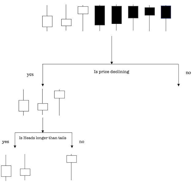
Let’s look at an example to better illustrate how one works.

Supposing our dataset consists of the price bars as indicated above. We have three falling candles and five rising candles (take bearish markets and bullish markets as our classes) and want to separate classes using their attributes. The attributes are price direction and comparison of head to tail length since these can be precursors to changes in direction. So how can we do this?

Price direction seems a straightforward attribute to separate by since white represents bearish candles and blue bullish. So, we can use the question, “Is price declining?” to separate the first junction. A junction in a tree as the point where branch splits into two —meeting criteria to choose the Yes branch and the No branch.

The No branch (rising candles) all have tails longer than heads so we are done there, but on the Yes branch this is not the case therefore there is more work to be done. On using the second attribute we ask, “Is heads longer than tails?” to make a second split.

The two declining candles with longer heads are under the Yes subbranch and one declining candle with a longer tail gets classified under the right subbranch. This decision tree was able to use the two attributes to divide up the data perfectly as per our criteria. 

In real trading systems tick volume, time of day and a host of other trading indicators can all be used in building a more comprehensive decision tree. Nonetheless the central premise of each question at a node is to find the one attribute the splits (or classifies) the data above into two dissimilar sets with created members of each set being similar.

Moving onto Random forest, like its name implies, consists of a huge number of individual decision trees that work as a group. For every tree in the random forest makes a class prediction and the class with the most votes is selected as the model’s prediction. The main concept behind random forest is easy to overlook but it’s very potent one — the wisdom of the masses. In making predictions uncorrelated trees outperform individual trees no matter how much data the individuals are trained on. Low correlation is the crux. The reason for this is that the trees protect each other from their individual errors according to Ton (as long as they don’t constantly all err in the same direction). For random forests to work though the prediction signal needs to be better than average and the perditions/ errors of each tree need to have a low correlation with each other.

As an example if you had two trade systems where in the first you get to place up to one thousand one dollar margin-orders in a year and the other you only get to place one 1000 dollar margin-order which one would you prefer assuming similar expectancy? For most people its the first system as it gives the trader 'more control'. 

So in what way do random forest algorithms ensure that the trait of each individual tree is not too correlated with the trait of any of the other trees in a forest? It could come down to two features:

2.0.1 Bagging

Decisions trees are very sensitive to training data with small changes potentially resulting in significantly different forests. Random forests use this by having each tree randomly sample the dataset while replacing, resulting in different trees. This process is known as bagging an abbreviation for bootstrap aggregation.

Notice that with bagging we are not substituting the training data into smaller sets but instead of the original training data, we take a random sample of size N with some replacements. The initial set size N is maintained. For example, if our training data was [U, V, W, X, Y, Z] then we might give one of our trees the following list [U, U, V, X, X, Z]. In both lists the size N (six) is kept and that “U” and “X” are both repeated in the randomly selected data.

2.0.2 Feature Randomness

Usually in a decision-tree, splitting the node involves considering every possible feature and selecting one that produces the widest distinction between the observations in the eventual left node vs. those in the eventual right node. On the other hand, in a random forest each tree can pick only from a random subset of features. This tends to force more variation within the forest and ultimately leads to lower correlation across trees and more diversification.

Let’s go through a visual example — in the picture above, the traditional decision tree (in blue) can select from all four features when deciding how to split the node. It decides to go with Feature 1 (black and underlined) as it splits the data into groups that are as separated as possible.

Now let’s take a look at our random forest. We will just examine two of the forest’s trees in this example. When we check out random forest Tree 1, we find that it it can only consider Features 2 and 3 (selected randomly) for its node splitting decision. We know from our traditional decision tree (in blue) that Feature 1 is the best feature for splitting, but Tree 1 cannot see Feature 1 so it is forced to go with Feature 2 (black and underlined). Tree 2, on the other hand, can only see Features 1 and 3 so it is able to pick Feature 1.

So in random forests, trees that are not only trained on sets of data (thanks to bagging) but also use variety of features in making decisions.

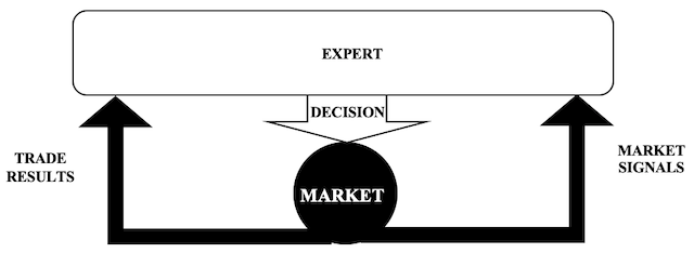
In using random forests our expert process past trade results and market signals to arrive at a buy or sell decision. In getting a signal and not just a screener from entropy we will consider separately the entropy of positive price bars and that of negative price bars within a recent set. 

The building and training of random forests will take place only on optimization with a single thread.

2.1 Expert Signal Class 

// wizard description start
//+------------------------------------------------------------------+
//| Description of the class                                         |
//| Title=Signals of'Shannon Entropy'                                |
//| Type=SignalAdvanced                                              |
//| Name=Shannon Entropy                                             |
//| ShortName=SE                                                     |
//| Class=CSignalSE                                                  |
//| Page=signal_se                                                   |
//| Parameter=Reset,bool,false,Reset Training                        |
//| Parameter=Trees,int,50,Trees number                              |
//| Parameter=Regularization,double,0.15,Regularization Threshold    |
//| Parameter=Trainings,int,21,Trainings number                      |
//+------------------------------------------------------------------+
// wizard description end
//+------------------------------------------------------------------+
//| Class CSignalSE.                                                 |
//| Purpose: Class of generator of trade signals based on            |
//|          the 'Shannon Entropy' signals.                          |
//| Is derived from the CExpertSignal class.                         |
//+------------------------------------------------------------------+
class CSignalSE : public CExpertSignal
   {
      public:
         
         //Decision Forest objects.
         CDecisionForest               DF;                                                   //Decision Forest
         CMatrixDouble                 DF_SIGNAL;                                            //Decision Forest Matrix for inputs and output
         CDFReport                     DF_REPORT;                                            //Decision Forest Report for results
         int                           DF_INFO;                                              //Decision Forest feedback

         double                        m_out_calculations[2], m_in_calculations[__INPUTS];   //Decision Forest calculation arrays

         //--- adjusted parameters
         bool                          m_reset;
         int                           m_trees;
         double                        m_regularization;
         int                           m_trainings;
         //--- methods of setting adjustable parameters
         void                          Reset(bool value){ m_reset=value; }
         void                          Trees(int value){ m_trees=value; }
         void                          Regularization(double value){ m_regularization=value; }
         void                          Trainings(int value){ m_trainings=value; }
         
         //Decision Forest FUZZY system objects
         CMamdaniFuzzySystem           *m_fuzzy;
         
         CFuzzyVariable                *m_in_variables[__INPUTS];
         CFuzzyVariable                *m_out_variable;

         CDictionary_Obj_Double        *m_in_text[__INPUTS];
         CDictionary_Obj_Double        *m_out_text;

         CMamdaniFuzzyRule             *m_rule[__RULES];
         CList                         *m_in_list;

         double                        m_signals[][__INPUTS];
         
         CNormalMembershipFunction     *m_update;
         
         datetime                      m_last_time;
         double                        m_last_signal;
         double                        m_last_condition;

                                       CSignalSE(void);
                                       ~CSignalSE(void);
         //--- method of verification of settings
         virtual bool                  ValidationSettings(void);
         //--- method of creating the indicator and timeseries
         virtual bool                  InitIndicators(CIndicators *indicators);
         //--- methods of checking if the market models are formed
         virtual int                   LongCondition(void);
         virtual int                   ShortCondition(void);

         bool                          m_random;
         bool                          m_read_forest;
         int                           m_samples;

         //--- method of initialization of the oscillator
         bool                          InitSE(CIndicators *indicators);
         
         double                        Data(int Index){ return(Close(StartIndex()+Index)-Close(StartIndex()+Index+1)); }
         
         void                          ReadForest();
         void                          WriteForest();
         
         void                          SignalUpdate(double Signal);
         void                          ResultUpdate(double Result);
         
         double                        Signal(void);
         double                        Result(void);
         
         bool                          IsNewBar(void);
  };

 

2.1.1 Signals

This entropy will be weighted by index for recency. 

            if(_data>0.0)
            {
               _long_entropy-=((1.0/__SIGNALS[i])*((__SIGNALS[i]-s)/__SIGNALS[i])*(fabs(_data)/_range)*(log10(1.0/__SIGNALS[i])/log10(2.0)));
            }
            else if(_data<0.0)
            {
               _short_entropy-=((1.0/__SIGNALS[i])*((__SIGNALS[i]-s)/__SIGNALS[i])*(fabs(_data)/_range)*(log10(1.0/__SIGNALS[i])/log10(2.0)));
            }

And it will also be weighted by magnitude of the price bars.

            if(_data>0.0)
            {
               _long_entropy-=((1.0/__SIGNALS[i])*((__SIGNALS[i]-s)/__SIGNALS[i])*(fabs(_data)/_range)*(log10(1.0/__SIGNALS[i])/log10(2.0)));
            }
            else if(_data<0.0)
            {
               _short_entropy-=((1.0/__SIGNALS[i])*((__SIGNALS[i]-s)/__SIGNALS[i])*(fabs(_data)/_range)*(log10(1.0/__SIGNALS[i])/log10(2.0)));
            }

Signal generated will be the negative bars entropy minus the positive bars’ entropy. The reasoning here is if the negative bars entropy exceeds that of the positive bars then we have less information regarding negative bars and therefore a short position than we do for the positive bars which likewise imply a long position. On the surface it does appear this will be a ‘dangerous’ trend following system! However because of the weightings attached above in computing the entropy, that may not be the case.

Signals will be updated when the long or short condition exceeds the open threshold as this implies a position will be opened. This will happen on timer so we’ll modify the wizard assembled expert to cater for this.

//+------------------------------------------------------------------+
//| "Timer" event handler function                                   |
//+------------------------------------------------------------------+
void OnTimer()
  {
   if(PositionSelect(Symbol()) && Signal_ThresholdClose<=fabs(filter0.m_last_condition))
     {
      filter0.ResultUpdate(filter0.Result());
     }
   //
   if(!PositionSelect(Symbol()) && Signal_ThresholdOpen<=fabs(filter0.m_last_condition))
     {
      filter0.SignalUpdate(filter0.m_last_signal);
     }
   ExtExpert.OnTimer();
  }

The source function in the class will only run on optimisation as already mentioned.

//+------------------------------------------------------------------+
//|                                                                  |
//+------------------------------------------------------------------+  
void CSignalSE::SignalUpdate(double Signal)
   {
      if(MQLInfoInteger(MQL_OPTIMIZATION))
      {
         m_samples++;
         DF_SIGNAL.Resize(m_samples,__INPUTS+2);
         
         for(int i=0;i<__INPUTS;i++)
         {
            DF_SIGNAL[m_samples-1].Set(i,m_signals[0][i]);
         }
         //
         DF_SIGNAL[m_samples-1].Set(__INPUTS,Signal);
         DF_SIGNAL[m_samples-1].Set(__INPUTS+1,1-Signal);    
      }
   }

 

2.1.2 Results

Results will be based on the profit of the last closed position.  

      if(HistorySelect(0,m_symbol.Time()))
      {
         int _deals=HistoryDealsTotal();
         
         for(int d=_deals-1;d>=0;d--)
         {
            ulong _deal_ticket=HistoryDealGetTicket(d);
            if(HistoryDealSelect(_deal_ticket))
            {
               if(HistoryDealGetInteger(_deal_ticket,DEAL_ENTRY)==DEAL_ENTRY_OUT)
               {
                  _result=HistoryDealGetDouble(_deal_ticket,DEAL_PROFIT);
                  break;
               }
            }
         }
      }
   
      return(_result);

And they will be updated when the long or short condition exceeds the close threshold as this implies a position will be closed. This also as above will happen on timer with the class function only updating decision forest files when optimising.

//+------------------------------------------------------------------+
//|                                                                  |
//+------------------------------------------------------------------+  
void CSignalSE::ResultUpdate(double Result)
   {
      if(MQLInfoInteger(MQL_OPTIMIZATION))
      {
         int _err;
         if(Result<0.0) 
         {
            double _odds = MathRandomUniform(0,1,_err);
            //
            DF_SIGNAL[m_samples-1].Set(__INPUTS,_odds);
            DF_SIGNAL[m_samples-1].Set(__INPUTS+1,1-_odds);
         }
      }
   }

2.1.3 Forest Writing

The forest will be written on tick prior to a read, so we modify the wizard assembled expert to accommodate this. 

//+------------------------------------------------------------------+
//| "Tick" event handler function                                    |
//+------------------------------------------------------------------+
void OnTick()
  {
   if(!signal_se.m_read_forest) signal_se.WriteForest();
   
   ExtExpert.OnTick();
  }

2.1.4 Forest Reading

The forest will be read on tester at the end of a tester pass so we modify the wizard assembled expert to accommodate this. 

//+------------------------------------------------------------------+
//| "Tester" event handler function                                  |
//+------------------------------------------------------------------+  
double OnTester()
   {
    signal_se.ReadForest();
    return(0.0);
   }

2.2 Expert Money Class

For this article we are also exploring creating a customized position sizing class to be used with the wizard. We will take the ‘Money Size Optimized’ class and modify it to normalize position sizes based on Shannon entropy. Our new interface will look like this: 

// wizard description start
//+------------------------------------------------------------------+
//| Description of the class                                         |
//| Title=Trading with 'Shannon Entropy' optimized trade volume      |
//| Type=Money                                                       |
//| Name=SE                                                          |
//| Class=CMoneySE                                                   |
//| Page=money_se                                                    |
//| Parameter=ScaleFactor,int,3,Scale factor                         |
//| Parameter=Percent,double,10.0,Percent                            |
//+------------------------------------------------------------------+
// wizard description end
//+------------------------------------------------------------------+
//| Class CMoneySE.                                                  |
//| Purpose: Class of money management with 'Shannon Entropy' optimized volume.          |
//|              Derives from class CExpertMoney.                    |
//+------------------------------------------------------------------+
class CMoneySE : public CExpertMoney
  {
protected:
   int               m_scale_factor;

public:
   double            m_absolute_condition;
   
                     CMoneySE(void);
                    ~CMoneySE(void);
   //---
   void              ScaleFactor(int scale_factor) { m_scale_factor=scale_factor; }
   void              AbsoluteCondition(double absolute_condition) { m_absolute_condition=absolute_condition; }
   virtual bool      ValidationSettings(void);
   //---
   virtual double    CheckOpenLong(double price,double sl);
   virtual double    CheckOpenShort(double price,double sl);

protected:
   double            Optimize(double lots);
  };

 The variable 'm_absolute_condition' will be the absolute value of the integer(s) returned by the 'LongCondition' and 'ShortCondition' functions. Since it is a normalised value, we can use its size to proportion our position size. This variable will be passed from the signal class to the money class via modifications to the wizard assembled expert.

//+------------------------------------------------------------------+
//| Global expert object                                             |
//+------------------------------------------------------------------+
CExpert ExtExpert;
CSignalSE *signal_se;
CMoneySE *money_se;

And on the tick function

//+------------------------------------------------------------------+
//| "Tick" event handler function                                    |
//+------------------------------------------------------------------+
void OnTick()
  {
   if(!signal_se.m_read_forest) signal_se.WriteForest();
   
   money_se.AbsoluteCondition(fabs(signal_se.m_last_condition));
   
   ExtExpert.OnTick();
  }

And the main modifications will be in the ‘Optimize’ function below: 

//+------------------------------------------------------------------+
//| Optimizing lot size for open.                                    |
//+------------------------------------------------------------------+
double CMoneySE::Optimize(double lots)
  {
   double lot=lots;
   
      //--- normalize lot size based on magnitude of condition
      lot*=(20*m_scale_factor/fmax(20.0,((100.0-m_absolute_condition)/100.0)*20.0*m_scale_factor*m_scale_factor));
      
      //--- reduce lot based on number of losses orders without a break
      if(m_scale_factor>0)
      {
         //--- select history for access
         HistorySelect(0,TimeCurrent());
         //---
         int       orders=HistoryDealsTotal();  // total history deals
         int       losses=0;                    // number of consequent losing orders
         CDealInfo deal;
         //---
         for(int i=orders-1;i>=0;i--)
         {
            deal.Ticket(HistoryDealGetTicket(i));
            if(deal.Ticket()==0)
            {
               Print("CMoneySE::Optimize: HistoryDealGetTicket failed, no trade history");
               break;
            }
            //--- check symbol
            if(deal.Symbol()!=m_symbol.Name())
               continue;
            //--- check profit
            double profit=deal.Profit();
            if(profit>0.0)
               break;
            if(profit<0.0)
               losses++;
         }
         //---
         if(losses>1){
         lot*=m_scale_factor;
         lot/=(losses+m_scale_factor);
         lot=NormalizeDouble(lot,2);}
      }
      //--- normalize and check limits
      double stepvol=m_symbol.LotsStep();
      lot=stepvol*NormalizeDouble(lot/stepvol,0);
      //---
      double minvol=m_symbol.LotsMin();
      if(lot<minvol){ lot=minvol; }
      //---
      double maxvol=m_symbol.LotsMax();
      if(lot>maxvol){ lot=maxvol; }
//---
   return(lot);
  }

 

3.0 MQL5 Wizard

We will assemble two expert advisors one with only the signal class we’ve created plus minimum volume trading for money management, and the second with both the signal and money management classes we’ve created.

4.0 Strategy Tester

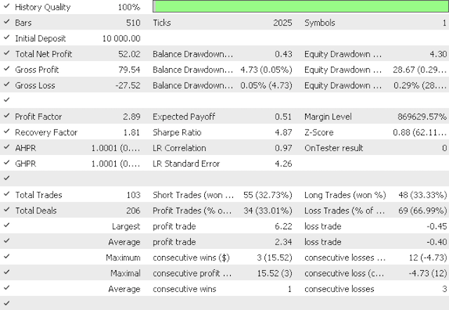
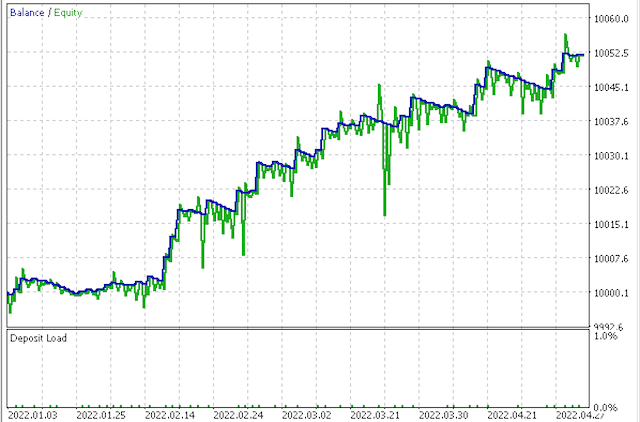
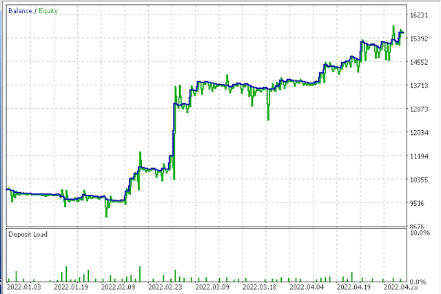
Running optimization for the first expert gives a profit factor of 2.89 and a Sharpe ratio of 4.87 vs a profit factor of 3.65 and Sharpe ratio of 5.79 from optimizing the second expert.

 

First report

 

 

First equity curve

 

Second report

 

 

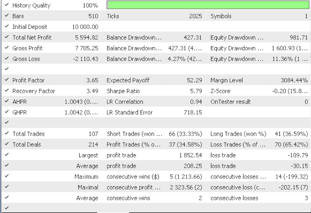
Second equity curve

 

5.0 Conclusion

The attached experts were optimized on open prices of the 4-hour timeframe for ideal take profit and stop loss levels.This means that you cannot replicate these results on a live account or even in strategy tester in every tick mode. That was not the point of the article. Rather than trying to come up with a grail that every one should replicate these series of articles seek to expose distinct ideas that can be customized further so every trader can come up with his edge. Markets on the whole are still too heavily correlated which is why looking for an edge can serve you well in high volatility. Thanks for reading!