
Data Science and ML (Part 36): Dealing with Biased Financial Markets

Contents
- Introduction
- Shortfalls of unbalanced target variable in machine learning
- Techniques to handle imbalanced dataset problem
- Choosing the proper evaluation metric
- An Expert Advisor(EA) for testing
- Oversampling techniques
- Undersampling techniques
- Hybrid methods
- Conclusion
Introduction
Different forex markets and financial instruments exhibit different behaviors at different times. While some financial markets such as stocks and indices are often bullish in the long run, others such as forex markets often display bearish behaviors and much more, this uncertainty adds complexity when trying to predict the market using Artificial Intelligence (AI) techniques and Machine Learning models (ML).

Let's take a couple of financial markets (trading symbols) and visualize 1000 bars market directions from the daily timeframe. If the closing price of a bar is above its opening we can label it as a bullish bar (1) otherwise, we can label it as a bearish bar (0).
import pandas as pd
import numpy as np

symbols = [
    "EURUSD",
    "USTEC",
    "XAUUSD",
    "USDJPY",
    "BTCUSD",
    "CA60",
    "UK100"
]

for symbol in symbols:

    df = pd.read_csv(fr"C:\Users\Omega Joctan\AppData\Roaming\MetaQuotes\Terminal\1640F6577B1C4EC659BF41EA9F6C38ED\MQL5\Files\{symbol}.PERIOD_D1.data.csv")
    df["Candle type"] = (df["Close"] > df["Open"]).astype(int)

    print(f"{symbol}(unique):",np.unique(df["Candle type"], return_counts=True))
Outcome.
EURUSD(unique): (array([0, 1]), array([496, 504]))
USTEC(unique): (array([0, 1]), array([472, 528]))
XAUUSD(unique): (array([0, 1]), array([472, 528]))
USDJPY(unique): (array([0, 1]), array([408, 592]))
BTCUSD(unique): (array([0, 1]), array([478, 522]))
CA60(unique): (array([0, 1]), array([470, 530]))
UK100(unique): (array([0, 1]), array([463, 537]))
As it can be seen from the outcome above, none of the trading symbols are perfectly balanced as there are different numbers of bears and bulls candles that appeared historically.
There is nothing wrong with the market being biased towards a specific direction but, this bias in historical data could cause some issues when training machine learning models, here is how:
Let's say we want to train some model on USDJPY based on the current dataset which has 1000 bars, we have 408 bearish candles (marked as 0) which is equal to 40.8% of all trading signals meanwhile we have 592 bullish candles (marked as 1) which amounts to 59.2% of all trading signals.
The presence of bullish signals which overwhelms the presence of bearish signals will be overlooked by machine learning models more often than not as the models tend to favor the most dominant class hence, make predictions in favor of the most dominant class.
Since all models aim to achieve the lowest possible loss value which is accompanied by the maximum accuracy value possible, the models will favor the bullish class which has occurred 59.2% out of 100% of the time as an easy way to hit the maximum accuracy value.
This isn't rocket science because based on just this simple information if you ignore all predictors and everything that's happening in the market just using this information when predicting the USDJPY you can say all the bars will be bullish all the time, and you will be correct approximately 59.2% of the time, not bad right? Wrong!
Because In doing so you will be assuming that what happened in the past is bound to happen again, something which is terribly incorrect and so damn wrong in this trading world.
As you can see having an unbalanced target variable in classification data for machine learning poses a problem, below are some of the shortfalls that come with this.
Shortfalls of Unbalanced Target Variables in Machine Learning
- Poor performance in the minority class
As I said earlier, the model biases predictions towards the majority class because it optimizes for overall accuracy. For example, In fraud detection data with (99% non-fraud, and 1% fraud) since most people are non-fraud, a model may predict non-fraud always and still get the 99% accuracy but, fail to detect fraud. - Misleading evaluation metrics
The accuracy value becomes unreliable, you can have a model with a joint accuracy of 72% unaware that one class was predicted 95% accurate while another class was 50% accurate. - Models overfitting on the majority class
The models could memorize noises from the majority class and make biased decisions instead of learning general patterns present in the predictors. For example, in medical diagnosis data with (95% healthy, and 5% diseased), the model may ignore the diseased cases entirely. - Poor generalization to unseen (real-world) data
In real-world data, distribution changes frequently and rapidly if a model was trained in a biased environment it is bound to fail sooner than later as it was trained on an unrealistic balance.
Techniques to Handle Imbalanced Dataset Problem
Now that we know the shortfalls that come with unbalanced (biased) target variable in a classification problem, let us discuss different ways to address this issue.
01: Choosing the Proper Evaluation Metric
The first technique to handle imbalanced data is choosing a proper evaluation metric, as said in the shortfalls, the accuracy of a classifier which is the total number of correct predictions divided by the total number of predictions can be misleading in unbalanced data.
In an imbalanced data problem, other metrics, such as precision which measure how accurate the classifier’s prediction of a specific class, and recall which measures the classifier’s ability to identify a class are much more useful than the accuracy metric.
When working with an imbalanced dataset most machine learning experts use the f1-score as it is more appropriate.
It is simply the harmonic mean of precision and recall, represented by the formula.

So, if the classifier predicts the minority class, but the prediction is erroneous and the false-positive increases, the precision metric will be low and so will the F1 score.
Also, if the classifier identifies the minority class poorly, then false negatives will increase, so recall and F1 score will be low.
The F1 score only increases if the number and overall prediction quality improve.
To understand this in detail, let's train a simple RandomForest classifier on the biased USDJPY instrument.
import pandas as pd
import numpy as np
from sklearn.model_selection import train_test_split
from sklearn.ensemble import RandomForestClassifier
from sklearn.metrics import classification_report

# Global variables

symbol = "USDJPY"
timeframe = "PERIOD_D1"
lookahead = 1
common_path = r"C:\Users\Omega Joctan\AppData\Roaming\MetaQuotes\Terminal\Common\Files"

df = pd.read_csv(f"{common_path}\{symbol}.{timeframe}.data.csv")

# Target variable

df["future_close"] = df["Close"].shift(-lookahead) # future closing price based on lookahead value
df.dropna(inplace=True)

df["Signal"] = (df["future_close"] > df["Close"]).astype(int)

print("Signals(unique): ",np.unique(df["Signal"], return_counts=True))

X = df.drop(columns=["Signal", "future_close"])
y = df["Signal"]

X_train, X_test, y_train, y_test = train_test_split(X, y, test_size=0.3, random_state=42, shuffle=False)

model = RandomForestClassifier(n_estimators=100,
                               max_depth=5,
                               min_samples_split=3,
                               random_state=42)

model.fit(X_train, y_train)
After training, we can save the model into ONNX format for later usage in MetaTrader 5.
from skl2onnx import convert_sklearn
from skl2onnx.common.data_types import FloatTensorType
import os

def saveModel(model, n_features: int, technique_name: str):

    initial_type = [("input", FloatTensorType([None, n_features]))]

    onnx_model = convert_sklearn(model, initial_types=initial_type, target_opset=14)

    with open(os.path.join(common_path, f"{symbol}.{timeframe}.{technique_name}.onnx"), "wb") as f:
        f.write(onnx_model.SerializeToString())
saveModel(model=model, n_features=X_train.shape[1], technique_name="no-sampling")
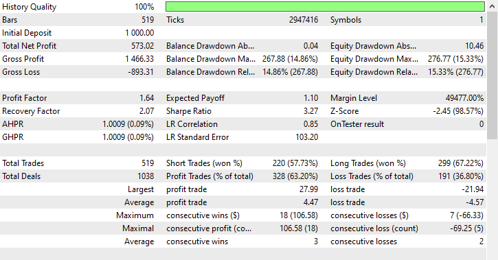
I had to use the classification report method to observe different metrics that come within Scikit-Learn.
Train Classification report
               precision    recall  f1-score   support

           0       0.98      0.41      0.57       158
           1       0.68      1.00      0.81       204

    accuracy                           0.74       362
   macro avg       0.83      0.70      0.69       362
weighted avg       0.81      0.74      0.71       362
Train classification report analysis
The overall training accuracy of the model is 0.74, which might seem decent at first glance, however, a closer look at the class-wise metrics reveals a significant imbalance in how the model performs across the two classes where class 0 has a very high precision of 0.98, but a low recall of 0.41 leading to a modest F1-score of 0.57.
This means that although the model is very confident when it predicts class 0, it misses a large number of actual class 0 samples, indicating poor sensitivity.
Class 1 on the other hand shows a recall of 1.00 and an F1-score of 0.81, but a relatively lower precision of 0.68.
This suggests the model is overly biased toward predicting class 1, possibly leading to a high number of false positives.
The perfect recall (1.00) for class 1 is a red flag as it likely indicates overfitting or a bias toward the majority class.
The model is predicting class 1 for almost everything and missing many actual class 0 samples, which is evident from class 0's poor recall value of 0.41.
Overall, these metrics not only show imbalance but also, they raise concerns about the model's generalization ability and its fairness across classes. Something is clearly off here.
Let us use the oversampling techniques to improve our model and find a predictive balance.
An Expert Advisor (EA) for Testing
There is always a difference between a machine learning model analysis results like the classification report above and the actual trading outcome from MetaTrader 5, Since we will be saving the model into ONNX format for later usage we can make a simple trading robot that takes a model trained on each resampling technique discussed in this article and use it to make trading decisions on the strategy tester on the training sample.
The data used was collected inside the file named Collectdata.mq5, a script that collects the training data from 01.01.2025 all the way back to 01.01.2023. You can find it in this articles' attachments.
Inside the Expert Advisor (EA) named Test Resampling Techniques.mq5, we initialize the model in ONNX format and then use it to make predictions.
#include <Random Forest.mqh>
CRandomForestClassifier random_forest; //A class for loading the RFC in ONNX format

#include <Trade\Trade.mqh>
#include <Trade\PositionInfo.mqh>

CTrade m_trade;
CPositionInfo m_position;

input string symbol_ = "USDJPY";
input int magic_number= 14042025;
input int slippage = 100;
input ENUM_TIMEFRAMES timeframe_ = PERIOD_D1;
input string technique_name = "randomoversampling";

int lookahead = 1;
//+------------------------------------------------------------------+
//| Expert initialization function                                   |
//+------------------------------------------------------------------+
int OnInit()
  {
//---

   if (!random_forest.Init(StringFormat("%s.%s.%s.onnx", symbol_, EnumToString(timeframe_), technique_name), ONNX_COMMON_FOLDER)) //Initializing the RFC in ONNX format from a commmon folder
     return INIT_FAILED;

//--- Setting up the CTrade module

   m_trade.SetExpertMagicNumber(magic_number);
   m_trade.SetDeviationInPoints(slippage);
   m_trade.SetMarginMode();
   m_trade.SetTypeFillingBySymbol(symbol_);

//---
   return(INIT_SUCCEEDED);
  }
//+------------------------------------------------------------------+
//| Expert deinitialization function                                 |
//+------------------------------------------------------------------+
void OnDeinit(const int reason)
  {
//---

  }
//+------------------------------------------------------------------+
//| Expert tick function                                             |
//+------------------------------------------------------------------+
void OnTick()
  {
//---

   vector x = {
      iOpen(symbol_, timeframe_, 1),
      iHigh(symbol_, timeframe_, 1),
      iLow(symbol_, timeframe_, 1),
      iClose(symbol_, timeframe_, 1)
   };

   long signal = random_forest.predict_bin(x); //Predicted class
   double proba = random_forest.predict_proba(x).Max(); //Maximum predicted probability

   MqlTick ticks;
   if (!SymbolInfoTick(symbol_, ticks))
      {
         printf("Failed to obtain ticks information, Error = %d",GetLastError());
         return;
      }

   double volume_ = SymbolInfoDouble(symbol_, SYMBOL_VOLUME_MIN);


   if (signal == 1)
     {
        if (!PosExists(POSITION_TYPE_BUY) && !PosExists(POSITION_TYPE_SELL))
            m_trade.Buy(volume_, symbol_, ticks.ask,0,0);
     }

   if (signal == 0)
     {
        if (!PosExists(POSITION_TYPE_SELL) && !PosExists(POSITION_TYPE_BUY))
            m_trade.Sell(volume_, symbol_, ticks.bid,0,0);
     }

//---

   CloseTradeAfterTime((Timeframe2Minutes(timeframe_)*lookahead)*60); //Close the trade after a certain lookahead and according the the trained timeframe
  }
//+------------------------------------------------------------------+
//|                                                                  |
//+------------------------------------------------------------------+
bool PosExists(ENUM_POSITION_TYPE type)
 {
    for (int i=PositionsTotal()-1; i>=0; i--)
      if (m_position.SelectByIndex(i))
         if (m_position.Symbol()==symbol_ && m_position.Magic() == magic_number && m_position.PositionType()==type)
            return (true);

    return (false);
 }
//+------------------------------------------------------------------+
//|                                                                  |
//+------------------------------------------------------------------+
bool ClosePos(ENUM_POSITION_TYPE type)
 {
    for (int i=PositionsTotal()-1; i>=0; i--)
      if (m_position.SelectByIndex(i))
         if (m_position.Symbol() == symbol_ && m_position.Magic() == magic_number && m_position.PositionType()==type)
            {
              if (m_trade.PositionClose(m_position.Ticket()))
                return true;
            }

    return (false);
 }
//+------------------------------------------------------------------+
//|                                                                  |
//+------------------------------------------------------------------+
void CloseTradeAfterTime(int period_seconds)
{
   for (int i = PositionsTotal() - 1; i >= 0; i--)
      if (m_position.SelectByIndex(i))
         if (m_position.Magic() == magic_number)
            if (TimeCurrent() - m_position.Time() >= period_seconds)
               m_trade.PositionClose(m_position.Ticket(), slippage);
}
//+------------------------------------------------------------------+
//|                                                                  |
//+------------------------------------------------------------------+

int Timeframe2Minutes(ENUM_TIMEFRAMES tf)
{
    switch(tf)
    {
        case PERIOD_M1:  return 1;
        case PERIOD_M2:  return 2;
        case PERIOD_M3:  return 3;
        case PERIOD_M4:  return 4;
        case PERIOD_M5:  return 5;
        case PERIOD_M6:  return 6;
        case PERIOD_M10: return 10;
        case PERIOD_M12: return 12;
        case PERIOD_M15: return 15;
        case PERIOD_M20: return 20;
        case PERIOD_M30: return 30;
        case PERIOD_H1:  return 60;
        case PERIOD_H2:  return 120;
        case PERIOD_H3:  return 180;
        case PERIOD_H4:  return 240;
        case PERIOD_H6:  return 360;
        case PERIOD_H8:  return 480;
        case PERIOD_H12: return 720;
        case PERIOD_D1:  return 1440; // 1 day = 1440 minutes
        case PERIOD_W1:  return 10080; // 1 week = 7 * 1440 minutes
        case PERIOD_MN1: return 43200; // Approx. 1 month = 30 * 1440 minutes

        default:
            PrintFormat("Unknown timeframe: %d", tf);
            return 0;
    }
}
Since we trained the model on the target variable based on the lookahead value of 1, we have to close the trade after the lookahead number of bars have passed on the current timeframe, by doing so we effectively ensure that the lookahead value is respected as we are holding and closing our trades according to the predictive horizon of the model.
Before we look at trading outcome on the models trained on the resampled data, let us observe the trading outcome from a model trained on the non-resampled training data (raw data).
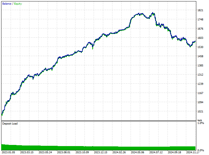
Tester configurations.
Inputs: technique_name = no-sampling.
Tester outcomes.
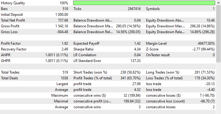
Despite the model being able to pick up some good signals and making some impressive trading outcomes with the overall profitable trades amounting to 62.24% of all the trades it took. If you look at the short and long trades won, you can see that there is a 1:4 ratio for shorts and long trades.
102 out of 519 trades taken were short trades, leading to a 70.59% winning rate whilst 417 out of 519 of the trades taken were long trades leading to a 60.19% winning accuracy, something is clearly off here because if we analyze the candle direction from January 1st, 2023 to January 1st, 2025 based on the lookahead value of 1.
print("classes in y: ",np.unique(y, return_counts=True))
Outcome.
classes in y: (array([0, 1]), array([225, 293]))
We can see that 225 were bearish price movements, whilst 293 were bullish movements, Since the majority of the candles moved in bullish direction on USDJPY in this 2 years period (from january 1st, 2023 to January 1st, 2025), any terrible model which favors the bullish movement could make a profit. It's not that hard.
Now we can understand that the only reason the model generated some profit was because it favored the long trades 4 times more than the short trades.
Since the market was bullish mostly in that period, it was able to generate some profits.
Let's proceed with resampling techniques and see how we can address this biased decision-making in our models.
Oversampling Techniques
Random oversampling
This is a technique used to address class imbalance in datasets by creating synthetic samples of the minority class.
It involves randomly selecting existing minority class examples and duplicating them to increase their representation in the training data, it aims to balance the class distribution in imbalanced datasets.
The most commonly used tool for this task is imbalanced-learn, below is a simple way to use it.
from imblearn.over_sampling import RandomOverSampler

print("b4 Target: ",np.unique(y_train, return_counts=True))

rus = RandomOverSampler(random_state=42)
X_resampled, y_resampled = rus.fit_resample(X_train, y_train)

print("After Target: ",np.unique(y_resampled, return_counts=True))
Outputs.
b4 Target:  (array([0, 1]), array([304, 395]))
After Target:  (array([0, 1]), array([395, 395]))
We can fit the resampled data to the same RandomForestClassifier we used before and observe the difference in the outcome compared to those achieved without resampling the data.
model.fit(X_resampled, y_resampled)
Model's evaluation.
y_train_pred = model.predict(X_train)

print("Train Classification report\n",classification_report(y_train, y_train_pred))
Outcome.
Train Classification report
               precision    recall  f1-score   support

           0       0.82      0.85      0.83       158
           1       0.88      0.86      0.87       204

    accuracy                           0.85       362
   macro avg       0.85      0.85      0.85       362
weighted avg       0.85      0.85      0.85       362
Amazing, these results indicate a significant improvement across all metrics. The F1-scores of 0.87 for both classes suggest that the model is making unbiased and consistent predictions, this points to a model with healthy generalization and well-distributed learning across the target classes.
Despite its simplicity and effectiveness, oversampling can increase the risk of overfitting by creating duplicate instances of the minority class, which may not add new information to the model.
Using the same tester configurations, we can test the model trained on this data on the Strategy tester.
Inputs: technique_name = randomoversampling.
Tester outcomes.
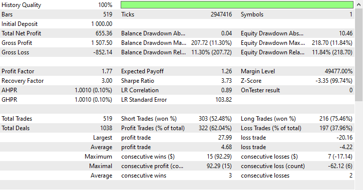
As you can see, we have improvements in all trading aspects, this model is more robust than the one trained with raw data. Now the robot opens more short trades and that has led to a significant reduction in the long trades.
Again in this training period the market exhibited 225 and 293 bearish and bullish movements respectively according to how we crafted the target variable, this new model trained on oversampled data appears to open 238 and 281 short and long trades respectively, this is a good sign that the model isn't biased as it makes decisions based on the learned patterns more than anything else.
Undersampling Techniques
There are a couple of undersampling techniques that we can use available in various Python modules. Some are:
Random Undersampling
This is a technique used to address class imbalance in datasets by reducing the number of samples from the majority class to balance it with the minority class.
It involves randomly or strategically removing samples from the majority class.
Similarly to how we applied oversampling, we can undersample the major class as follows.
from imblearn.under_sampling import RandomUnderSampler

print("b4 Target: ",np.unique(y_train, return_counts=True))

rus = RandomUnderSampler(random_state=42)
X_resampled, y_resampled = rus.fit_resample(X_train, y_train)

print("After Target: ",np.unique(y_resampled, return_counts=True))
Outcome.
b4 Target:  (array([0, 1]), array([304, 395]))
After Target:  (array([0, 1]), array([304, 304]))
Random undersampling and other under sampling can degrade model performance by removing informative majority class samples, leading to a less representative training set. This could potentially cause underfitting of the model.
This technique improved the performance of the model on the training data for both classes.
Train Classification report
               precision    recall  f1-score   support

           0       0.76      0.90      0.82       158
           1       0.91      0.78      0.84       204

    accuracy                           0.83       362
   macro avg       0.83      0.84      0.83       362
weighted avg       0.84      0.83      0.83       362
Using the same tester configurations, we can test the model trained on this data on the Strategy tester.
Inputs: technique_name = randomundersampling.
Tester outcomes.

This technique produced 282 and 237 short and long trades respectively, despite this model favoring short trades over long trades something which did not appear on the market, it was still able to make more profits than the biased model trained with raw data, and the oversampled model which favored bullish movements.
These outcomes from the model tells us that, we can make profits from the market on both directions regardless on what happened historically.
Tomek Links
Tomek links refer to a pair of instances from different classes that are very close to each other, often considered nearest neighbors. Here is the simple explanation on how the tomek links technique operates for undersampling machine learning data.
Imagine we have two points A and B from different classes, A belongs to the majority class whilst B belongs to the minority class (or viceversa).
If these two points (A and B) are close to each other (neighbors) then an observation from the majority class (A in this case) will be deleted.
This technique helps in cleaning the decision boundaries and make the classes more distinct while still removing some samples from the majority class.
from imblearn.under_sampling import TomekLinks

tl = TomekLinks()
X_resampled, y_resampled = tl.fit_resample(X_train, y_train)

print(f"Before --> y (unique): {np.unique(y_train, return_counts=True)}\nAfter  --> y (unique): {np.unique(y_resampled, return_counts=True)}")
Outputs.
Before --> y (unique): (array([0, 1]), array([304, 395]))
After  --> y (unique): (array([0, 1]), array([304, 283]))
This technique can lead to impressive balanced predictive outcomes from the model but, it is limited to binary classification, less effective in highly overlapping data, and just like other sampling techniques, it can lead to data loss.
This technique also had a better performance on the training data.
Train Classification report
               precision    recall  f1-score   support

           0       0.69      0.94      0.80       158
           1       0.93      0.68      0.78       204

    accuracy                           0.79       362
   macro avg       0.81      0.81      0.79       362
weighted avg       0.83      0.79      0.79       362
Using the same tester configuration we can test the model trained on this data on the Strategy tester.
Inputs: technique_name = tomek-links.
Tester outcomes.

Similarly to the Random undersampling technique, Tomek links favored short trades as it opened 303 short trades while 216 long trades were opened, it was able to make profits regardless.
Cluster centroids
This is an under-sampling technique where the majority class is reduced by replacing its samples with the centroids of clusters (usually from K-means clustering).
It works as follows.
- K-means clustering is applied to the majority class.
- The K-number of desired samples are chosen.
- The majority of samples in the class are replaced with k cluster centers.
- This outcome is combined with the minority class to create a balanced dataset.
from imblearn.under_sampling import ClusterCentroids

cc = ClusterCentroids(random_state=42)
X_resampled, y_resampled = cc.fit_resample(X, y)

print(f"Before --> y (unique): {np.unique(y_train, return_counts=True)}\nAfter  --> y (unique): {np.unique(y_resampled, return_counts=True)}")
Outputs.
Before --> y (unique): (array([0, 1]), array([158, 204]))
After  --> y (unique): (array([0, 1]), array([225, 225]))
Below is the outcome of the model on the training data undersampled using cluster centroids.
Train Classification report
               precision    recall  f1-score   support

           0       0.64      0.86      0.73       158
           1       0.85      0.62      0.72       204

    accuracy                           0.73       362
   macro avg       0.75      0.74      0.73       362
weighted avg       0.76      0.73      0.73       362
So far, this technique is the one with the least accuracy value, a 0.73 value could indicate that the model is less overfitted than the previous ones so it might as well be the best possible model so far, let us observe its accuracy on a trading environment.
Inputs: technique_name = cluster-centroids.
Tester outcomes.

This technique provided the highest number of profit trades 343 trades out of 519, a 66.09% accuracy as its profits nearly reached the initial deposit. Despite the model favoring more short trades, it was very accurate in predicting the bullish signals leading to a whooping 75.97% out of 100% winning long positions.
Hybrid Methods
SMOTE + Tomek Links
Applies SMOTE first, then cleans up noise with Tomek Links.
from imblearn.combine import SMOTETomek

smt = SMOTETomek(random_state=42)
X_resampled, y_resampled = smt.fit_resample(X_train, y_train)

print(f"Before --> y (unique): {np.unique(y_train, return_counts=True)}\nAfter  --> y (unique): {np.unique(y_resampled, return_counts=True)}")
Outputs.
Before --> y (unique): (array([0, 1]), array([158, 204]))
After  --> y (unique): (array([0, 1]), array([159, 159]))
Below is the outcome of the model trained on training data resampled by this technique.
Train Classification report
               precision    recall  f1-score   support

           0       0.74      0.73      0.73       158
           1       0.79      0.80      0.80       204

    accuracy                           0.77       362
   macro avg       0.77      0.77      0.77       362
weighted avg       0.77      0.77      0.77       362
Below are the trading outcomes.
Inputs: technique_name = smote-tomeklinks.
Tester outcomes.
220 and 299 short and long trades respectively, not bad.
SMOTE + ENN (Edited Nearest Neighbors)
SMOTE generates synthetic samples, then ENN removes misclassified samples.
from imblearn.combine import SMOTEENN

sme = SMOTEENN(random_state=42)
X_resampled, y_resampled = sme.fit_resample(X_train, y_train)

print(f"Before --> y (unique): {np.unique(y_train, return_counts=True)}\nAfter  --> y (unique): {np.unique(y_resampled, return_counts=True)}")
This technique removed a huge chunk of data, the training data was reduced to a total of 61 samples.
Before --> y (unique): (array([0, 1]), array([158, 204]))
After  --> y (unique): (array([0, 1]), array([37, 24]))
Below is the classification report on a training sample.
Train Classification report
               precision    recall  f1-score   support

           0       0.46      0.76      0.58       158
           1       0.63      0.32      0.42       204

    accuracy                           0.51       362
   macro avg       0.55      0.54      0.50       362
weighted avg       0.56      0.51      0.49       362
The resulting model is a bad one as expected because it was trained on 61 samples total, insufficient data for any model to learn meaningful patterns. Let us observe the trading outcomes.
Inputs: technique_name = smote-enn.
Tester outcomes.
This technique didn't help at all, it even made matters worse. It introduced biased trading outcomes as the robot opened 180 out of 519 buy trades and 339 sell trades.
This doesn't mean the technique is bad after all it's just not the optimal one in this situation.
Conclusion
We live in non-perfect world, not all the phenomena that occurs have suitable explanations or a clear path, this is true in the trading world where markets change rapidly and frequently causing most of our strategies to become obsolete instantly.
While we cannot control what happens in the market the best thing we can do is to ensure that we have atleast robust trading systems and strategies designed to work in extreme conditions.
Since history doesn't always repeat itself, it is a good thing to ensure that we have unbiased trading systems designed to work in any market by acknowledging the patterns that emerged in the market previously but not relying too much on them for making trading decisions. As helpful as these techniques can be, you have to be mindful of their drawbacks and tradeoffs that come with using resampling techniques for your machine learning data. Such drawbacks include the risk of overfitting from oversampling, the potential loss of valuable information when undersampling, and the introduction of noise or bias if the resampling is not done carefully.
Striking the right balance is key to building robust models that generalize well to unseen market conditions.
Best regards.
Attachments Table
| Filename | Description/Usage |
|---|---|
| Experts\Test Resampling Techniques.mq5 | An Expert Advisor (EA) for deploying .ONNX files in MQL5 |
| Include\pandas.mqh | Python-Like Pandas library for data manipulation and storage |
| Scripts\Collectdata.mq5 | A script for collecting the training data |
| Common\*.onnx | Machine learning models in ONNX format |
| Common\*.csv | Training data from different instruments machine learning usage |
Warning: All rights to these materials are reserved by MetaQuotes Ltd. Copying or reprinting of these materials in whole or in part is prohibited.
This article was written by a user of the site and reflects their personal views. MetaQuotes Ltd is not responsible for the accuracy of the information presented, nor for any consequences resulting from the use of the solutions, strategies or recommendations described.

 Building a Custom Market Regime Detection System in MQL5 (Part 1): Indicator
- Free trading apps
- Over 8,000 signals for copying
- Economic news for exploring financial markets
You agree to website policy and terms of use
Thanks, You Omega , Appreciate you putting this together , Bais is something we all fear. I have downloadted the attachments , Could I suggest it includes all the required componets . Thankfully you have the github so I was able to find and install the prerequisites (preprossing.mqh, plots.mqh ,Matrixextend.mqh, metrics.mqh and Random Forext.mqh). Unfortunately I then am stuck with the message ' Init - Undeclared Identifier ' from the line if (!random_forest.Init(StringFormat("%s.%s.%s.onnx", symbol_, EnumToString(timeframe_), technique_name), ONNX_COMMON_FOLDER)) //Initializing the RFC in ONNX format from a common folder. I checked and I do have USDJPY.PERIOD_D1.randomundersampling.onnx in MQL5\Common folder
The required components are the latest version of everything imported inside the notebook, you can do pip install without worrying about the versions conflicts. Alternatively, you can follow the link on the attachments table, it takes you to Kaggle.com where you can edit and modify the code.
Undeclared identifier, could mean a variable or an object isn't defined. Inspect your code or DM me send me a screenshot of the code.