Using spreadsheets to build trading strategies

Introduction

Spreadsheets are a fairly old invention. Modern programs of this type have tremendous power and allow you to visually analyze data presented in tabular form. The analysis can be done from different angles and is performed quite quickly. It includes graphs, summary tables, what-if analysis, conditional cell formatting and much more.

I suggest testing some of this power to analyze custom strategies.

Personally, I use LibreOffice Calc because it is free and it works wherever I work :-) However, the same approach works for other spreadsheets: Microsoft Excel, Google Sheets, etc. Currently, they all allow converting into each other and feature the same principles of constructing equations.

So, I assume, you have some kind of spreadsheet program. You also have data in a text file format (*.txt or *.csv) you want to analyze. The article briefly describes how to import such files. I will use history from MetaTrader terminal, however, any other data will do, like Dukascopy or Finam. Obviously, you should have a strategy to configure signals. This is all that is required to apply article propositions in trading.

I hope, the article will be useful to different categories of traders, so I will try to write it so that it is understandable even for people who have never seen programs of this type before. At the same time, it will cover a range of issues even some experienced traders are not familiar with.

A quick glance at tables — for beginners

Figure 1 shows a typical spreadsheet program window.

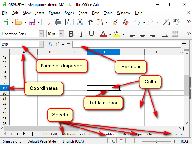
Figure 1. A typical spreadsheet program window

Any table is presented as a set of "sheets". You can think of them as separate "tabs" for different tasks.

Each sheet consists of "cells". Each cell is essentially a small but very powerful calculator.

To let the program understand which cell we want to process right now, each cell features coordinates, like on a chessboard or in a Battleship board game. These coordinates together define a unique cell "address". The address consists of a column number or name and a row number (for example, Figure 1 shows the "D19" cell highlighted by the table cursor). It can be seen both in the highlighted coordinate names and in the name line.

In addition to coordinates, an address may contain the name of the sheet and even the name of the table file. The same address is usually used as the name of the cell. But, if you wish, you can set your own names to make clear what exactly this cell or range of cells stores. You can view (and change) these names in the name line.

A cell may contain either simple data (like quotes or volumes) or "formulas" used to calculate its value.

The contents of a highlighted cell can be seen (and changed) in the "equation line".

To edit a cell value, double-click on it or make your corrections in the formula line. You can also highlight a cell and press F2.  If you need to create a new text, you may highlight a cell and start typing right away. However, keep in mind that all previous data will be deleted from the cell.

You can cancel editing without saving it by pressing ESC (upper left corner of the keyboard). Confirm editing by hitting Enter (the cursor is moved down) or Tab (the cursor is moved aside).

If several cells are highlighted, Enter and Tab work only in the highlighted fragment. This can be used to speed up work.

As for other buttons and menus, I think, they are pretty easy to grasp.

Getting started: importing quotes

Let's prepare data to test strategies. As I said, I will take data from the terminal. To do this, press Ctrl+S in any chart window or select File -> Save in the terminal menu. The terminal offers the usual system window to enter the file name and path.

If the file extension is *.csv, then usually all goes fine. If it is *.txt, then in most cases, you need to right-click it and select "Open with" ->"Choose another app" or open the spreadsheet app first and open the file from it, since the system tends to open files with this extension using Notepad or other word processor by default.

In order to convert numbers, select the appropriate column in the conversion window. Then indicate the separator of the integer and fractional parts, as well as the separator of the digit groups (for volumes) if necessary. In Excel, this is done using the "More ..." button. In Calc, select English USA from the Column Type list.

There is yet another nuance. After a successful import, it makes sense to leave 5-7 thousand rows in the table. The fact is that the more data there is, the more difficult it is for the program to calculate the result of each cell. At the same time, the estimation accuracy increases insignificantly. For example, when comparing the verification results for data of 5,000 and 100,000 rows, the results differed by only 1%, while the computation time in the latter case increased significantly.

Some keyboard shortcuts for working with tables

Shortcut	Action
Ctrl + arrows	Go to the nearest continuous data row border
Tab	Confirm input and go to the right cell
Shift + Tab	Confirm input and go to the left cell
Enter	Confirm input and go to the cell below
Shift + Enter	Confirm input and go to the cell above
Ctrl + D	Fill in highlighted columns from top to bottom
Shift + Ctrl + arrows	Highlight from the current position to the end of the continuous range

How to fill a long column with the same equation

For small ranges, you can use the method shown in Figure 2: move the mouse to the "selection marker" (the square in the lower right corner of the table cursor). When the mouse cursor turns into a thin cross, drag this marker to the desired row or column.

Figure 2. Filling in by dragging

However, for large amounts of data this would be highly inconvenient.

Therefore, use any of the methods below.

Method 1. Limiting the range

The sequence of actions is shown in Figure 3.

Figure 3. Filling in by limiting the range

1. Enter the desired equation in the top cell of the range and confirm the entry.
   
2. Move to the bottommost cell of the range using the name field.
   
3. Press Ctrl + Shift + up arrow to move to the topmost cell in the range and select all intermediate cells.
4. Press Ctrl + D to fill cells with data.

A small disadvantage of the method is that you need to know the number of the lowest row of the range.

Method 2. Using an adjacent continuous range

The sequence of actions is shown in Figure 4.

Figure 4. Filling in by using an adjacent range

1. Select the cell with a necessary equation.
2. Press Shift + left arrow to select an adjacent cell.
3. Press Tab to move the table cursor to the left cell. Here we use the ability of the table cursor to move only within the applied selection.
4. Ctrl + Shift + down arrow — select two columns to the lowest row of the continuous range.
5. Shift + right arrow — deselect the left column. The right one remains selected.
6. Ctrl + D — fill in the column with data.

Note the contents of the equation line in the figure. When copying the equation containing the link to another cell, this link automatically changes depending on the cursor position. Therefore, such a link is called "relative".

If you need the link to the cell to remain constant during copying, select the link and press F4. $ sign appears before the row number and column name, and the value does not change when copying the equation.

Sometimes, you may want only a certain column or row to remain intact, rather than the entire link. In this case, leave $ sign in the UNchangeable part only (you can press F4 one or two more times).

Now, after we have mastered the basic methods of accelerating our work, it is time to move on to the strategy itself.

Strategy

Let's use the strategy implemented in the standard "Examples\Moving Average" EA.

A position is opened if:

1. There are no positions and
2. The candle crosses the Moving Average with its body (Open — on one side of the МА, Close — on the other.)

A position is closed if:

1. There is an open position and
2. The candle crosses the MA in the opposite direction to the opening.

Adding indicator data

The distinguishing feature of calculating using spreadsheets is that subtotals of calculations, as a rule, need to be saved separately. This makes it easier to understand equations and detect errors, and also simplifies building equations based on data from adjacent cells. Besides, such a "fragmentation" sometimes gives rise to new ideas.

But let's get back to our task.

After importing and a little formatting, my original quotes look like this (Figure 5):

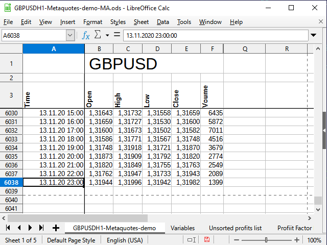
Figure 5. Original quotes

Note the blank row between the name of the entire table and the column names. This row allows the spreadsheet processor to treat the two blocks as separate tables, and therefore I can combine the cells for the top range, but still use different filters for the bottom range — and they will not interfere with each other. Removing the line may cause issues.

I have fixed the first rows and columns to hide the information that is unnecessary at the moment, but all the data is still present in the table (see the help for your spreadsheet processor on how to do this).

Time and date are in the column A, opening prices are in the column B, etc. The last row of the table is numbered 6038.

The first step to building a strategy is building an indicator. In order for the indicator to be customizable, let's add another sheet and create a table of variables there. We will assign a proper name to each variable using the name line so that it is clear what and where to take when preparing the equations.

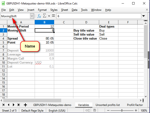
Figure 6. Variable sheet

Now let's go back to the data sheet. First, write the quote index in the list in the G column to slightly simplify the final equation. It is equal to the row index minus 3:

=ROW()-3

After writing the equation in the G4 cell, extend it to all lower cells so that the MA calculation equation remains universal. If MA (offset + period) exceeds the existing data, then the average calculation becomes meaningless.

The SMA calculation equation itself is written in Н4 of the main data sheet and looks as follows:

=IF( G4>(MovingPeriod+MovingShift), AVERAGE( INDIRECT( "E" & ( ROW()-MovingShift-MovingPeriod) & ":" & "E" & ( ROW()-MovingShift) ) ), "" )

When entering equations requiring links to other cells, you can specify the cells by mouse.

The current equation starts from calling the IF() function. As you might guess, this is the condition check function. All boolean expressions, like And, Or, Not, will also be functions in case they are needed later.

When calling functions, arguments are specified in parentheses and separated by commas (as in this case) or semicolons.

The IF function accepts three arguments: condition, value if condition is true and value if condition is false.

In this case, I used it to check if there is enough data to calculate a full-fledged point for the MA curve. If there is not enough data, simply save an empty string. Otherwise, calculate the average value from some range.

The Indirect function returns the value (or several values) from the range set by the text string. This is exactly what I need, since the addresses of the required ranges for calculating the average should be formed based on the input values.

The & symbol in spreadsheet programs denotes the concatenation of two rows. Thus, I have "combined" the address from several parts. The first part is a column name the closing prices ("Е") are located in, while the second one is a "remote" address calculated as the current row number minus the averaging length and minus the shift. The third piece of this expression is the colon sign indicating the continuity of the range. It is followed by the column and row names considering the shift. I decided not to highlight them too brightly. I hope, the ampersand cut-ins will be helpful in figuring it out.

The equation should be extended to all the rows below.

As a result, we get something like this:

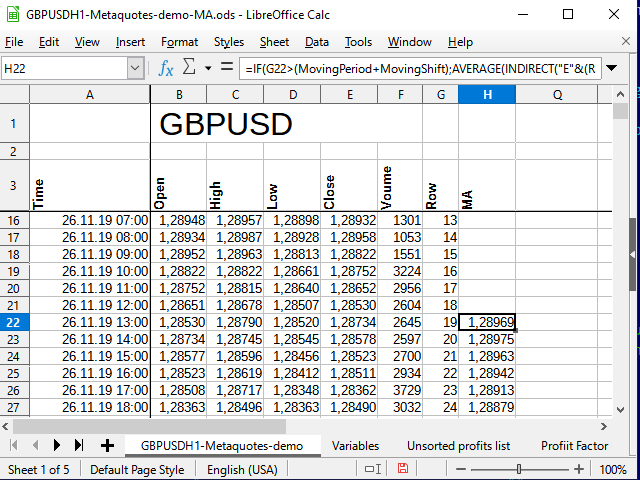
Figure 7. The table after adding МА calculations

As we can see, the numbers in the Н column started to appear only in the row 22 (the 19th entry). The reason for this is explained in Figure 6.

Now we have the initial data, as well as the indicator data. It is time to implement the strategy.

Implementing the strategy

We will implement the strategy in the form of simple signals. If МА is crossed downwards, the cell receives the value of "-1", otherwise — "1". If there are no intersections at the moment, the cell contains the empty string value.

Move to cell I4. The basic equation for the cell looks like this:

=IF( AND( B4>H4,E4<H4 ),-1 , IF( AND( B4<H4,E4>H4 ), 1 , "") )

You can check it on the graph, it works. But this is a simple reversal equation. It does not allow to track the deal status. You can experiment with it and get interesting results, but our task now is to implement the strategy described at the beginning of the article. Therefore, we need to record the deal status at each bar (in each line).

J column is quite suitable for this. The equation in J4 cell looks as follows:

=IF(AND(I4=-1,J3=""), -1 ,IF(AND(I4=1,J3=""), 1 ,IF(OR(AND(I4="",J3=1),AND(I4="",J3=-1),I4=J3), J3 ,"")))

If an event (intersection) has occurred, check the status of the previous deal. If the deal is open and the intersection occurs in the opposite direction, close it. If the deal is closed, open it. In all other cases, simply save the status.

Let's introduce another column featuring signals in order to clearly see where we would have bought and sold if we had implemented this strategy in the period our data corresponds to, and also in order to make it convenient to analyze the strategy.

Signal names can be taken from the help, which can be created on the variable sheet.

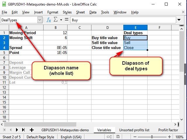
Figure 8. The Variable sheet after adding the help for deal names

Note the name line: here I set the name to the entire selected range, rather than to a single cell.

Now we can write the following in К4 cell of the main sheet (with data):

=IF(AND(J3=1,J2=""),INDEX(DealTypes,1),IF(AND(J3=-1,J2=""),INDEX(DealTypes,2),IF(OR(AND(J3="",J2=1),AND(J3="",J2=-1)),INDEX(DealTypes,3),"")))

The deal is opened after a signal at the opening of the next candle. Therefore, pay attention to the shift of the indices in this equation.

If there has been no deal (the previous cell in the status column is empty) and a signal has arrived, specify what deal type should be made. If the deal has been opened, close it according to the signal.

The Index function accepts the range the search is to be performed in as the first parameter. In our case, it is set by the name. The second parameter is the index of the row within the range. If the range consists of several columns, set the necessary column. If several ranges are specified separated by semicolons, set the range index starting from 1 as well (the third and fourth parameters, respectively).

As a result, after extending this equation to all the cells below and applying conditional formatting (for more visual appeal, since formatting is not needed during analysis), we will get approximately the following:

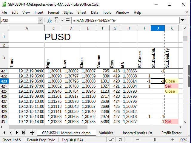
Figure 9. Signals for deals

Analyzing the strategy

To analyze the strategy profitability, I need to calculate the distance traveled by the price during the trade period. The easiest way to do this is in several stages.

First, select the deal price. If a deal is opened, set the price in the column next to the signal (L) and copy it to each subsequent cell until the deal is closed. If there is no deal, then an empty line is written to the cell. The equation in L4 cell:

=IF(K4=INDEX(DealTypes;1);B4+Spread;IF(K4=INDEX(DealTypes;2); B4 ;IF(OR(K4=INDEX(DealTypes;3);N(L3)=0); "" ;L3)))

If the signal cell (К4) features the word "Buy", the deal open price is equal to the candle open price plus spread. If the word is "Sell", simply write the candle open price, if "Close" (or the previous column cell does not contain a number) — an empty string, and if the previous cell of the same column is a number, while the signal column contains no words, simply copy the previous cell.

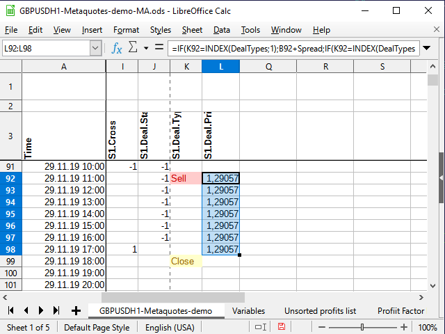
Figure 10. Deal open price

Thus, we will be able to easily calculate the deal profit at the moment of closure.

Be sure to extend the equation below.

We could immediately calculate the difference between the opening and closing prices in the adjacent column. But instead, we will do something more tricky. We will calculate the difference in the N column to be able to sort out unique data only and calculate its frequency afterwards.

In the current simplest assessment case, I will not use any money management since my objective is to evaluate the strategy efficiency. Therefore, it is enough to calculate the price difference in pips. For example:

=IF(K4=INDEX(DealTypes;3);IF(I3=-1;ROUND((B4-L3)/Point);ROUND((L3-B4)/Point)); "" )

It is clear that instead of checking the average condition, we could simply multiply (B3-L3)*I3 , but this would be less visually clear for beginners.

And now it is the time for the mentioned trick. In М column, number all unique entries about the deal range leaving non-unique ones without numbers.

=IF(N4<>"";IF(COUNTIF(N$3:N4;N4)=1;MAX(M3:M$4)+1;"");"")

The external condition is quite clear: if the right cell (N4) is not empty, check whether it is unique and number it if necessary, otherwise leave an empty string.

But how does the numbering work?

The Countif function counts the amount of numbers within the specified range provided that the cell value corresponds to the condition specified in the second parameter. Suppose that the equation is calculated for the M71 cell. The N71 cell contains the number 531 (see Figure 11). This number has never been seen before.

If the action sign is not indicated in the condition cell, it is assumed that we want to check the equality of two values. The number is equal to itself (N71=N71), so let's try to calculate. The calculation always starts from the N$3 cell (note the dollar sign before the number of three) and up to the current cell (no dollar sign in the equation). View the entire N$3:N71 range and try to count the total number of 531 numbers in this range. Since there were no such numbers before, the total number is 1 (just what was found now). This means the condition is fulfilled: the function result is 1. Therefore, we take the following range: the column the equation is located in starting from the very first cell with numbers (M$4) up to the cell preceding the current one (M70). If there were any numbers there before, take the largest of them and add 1 to them. If not, the largest one is 0, and, accordingly, the first sequence number is ready!

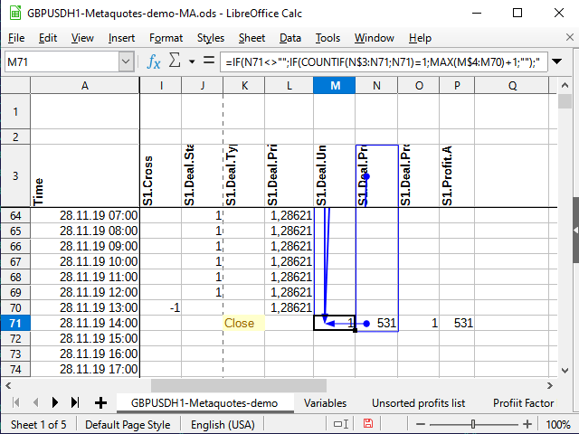
Figure 11. Numbering. Affecting cells (range final point)

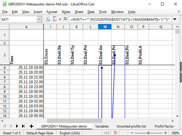
Figure 12. Numbering (range starting point)

In Figure 11, I tried to use the built-in analysis tool that shows the cells that are affecting a given cell. The dot with the arrow indicates the beginning of the ranges or "exact" cells, while the rectangles indicate the ranges. I have attached Figure 12 for clarity to make it evident that the arrow is continuous and starts exactly at N$3, as well as to make the starts of the ranges, in which the comparisons are done, visible.

Besides, I will add two more columns of values: result type and deal "module".

For the result types, I use numbers: buy deal — 1, sell deal — 2. In this case, the result can be positive or negative, depending on whether we received a profit or loss as a deal result. This will make the final analysis equations shorter.

Here is the equation written to О4 cell:

=IF(AND(N(N4)>0;I3=-1); 1 ;IF(AND(N(N4)<0;I3=-1); -1 ;IF(AND(N(N4)>0;I3=1); 2 ;IF(AND(N(N4)<0;I3=1); -2 ;""))))

The "module" is simply the amount of profit or loss without considering the sign. It is a description of how far the price went in one direction until the deal closure signal arrived. This can help you choose stop losses and take profits (even if they are not needed for the original strategy).

The "module" equation is quite primitive and set in P4:

=IF(N4<>"";ABS(N4);"")

In order to build a frequency (probabilistic) graph, it is better to arrange the deal result data in ascending order. Copy them to another sheet since the original data is sorted by time and cannot be sorted otherwise.

Given that each unique profit result has its own unique number (М column), there are at least two ways to copy unsorted data to a new sheet.

One of them is to simply select "non-empty" cells using a standard filter in the М column and then copy the data from the N column and paste it to another sheet using the special paste (values only).

The second method is to use the equation. Its advantage is that the data itself will change when the original data (the same variables or some other ones if you decide to use other test range) changes. The disadvantage is that it will probably still be impossible to sort. You will still have to use Copy/Paste to sort it.

It is more convenient for me when sorted and unsorted data are on the same sheet, because it takes a little less actions to copy the data. Therefore, I will show an option, in which unsorted data is copied using the equation and then copied again manually for sorting.

On the new Profit data sheet, create the equation in А2:

=VLOOKUP( ROW(1:1);'GBPUSDH1-Metaquotes-demo'.$M$3:$N$6038; 2 )

The Row(1:1) function returns the number of the first row. When filling the cells downwards, the row number changes, and, accordingly, the number of the second, third row, etc. is displayed.

Vlookup looks for some value (the first parameter) in the first column of the range (the second parameter), and then returns the value located in the same detected row, albeit in the column specified in the third parameter (in our case, this is the column 2 of the specified range). In other words, all numbered (unique) numerical values are copied from the N column starting with 1.

After defining the last number on the main sheet using the standard filter, you can copy all the remaining data using the range limitation method.

The following actions are shown in the Figure 13 animation.

Figure 13. Copying data for sorting

Now we need to describe the frequency of profitable and unprofitable trades, i.e. build a probability series.

In D2 cell of the same sheet (Profit data), we can write the following equation:

=COUNTIF('GBPUSDH1-Metaquotes-demo'.$N$4:$N$6038;C2)/COUNT('GBPUSDH1-Metaquotes-demo'.$N$4:'GBPUSDH1-Metaquotes-demo'.$N$6038)

It describes the frequency (or probability) of each profit value.

The Count function calculates the number of numerical values in the interval, Countif does the same if the condition is met (in this case, only the cells whose value is equal to the value in the C column cell are calculated).

It is usually recommended doing interval variation series. In theory, we can say that the number of deals can be quite large.

The size of the interval is recommended to be calculated using the equation:

=(MAX($'Profit data'.C2:$'Profit data'.C214)-MIN($'Profit data'.C2:$'Profit data'.C214))/(1+3,222*LOG10(COUNT('GBPUSDH1-Metaquotes-demo'.$N$4:'GBPUSDH1-Metaquotes-demo'.$N$6038)))

I put this equation in 'Variables'.E7 cell and named it "Interval". The interval turned out to be too large. It was unclear for me how probabilities were distributed in general, so I divided it by 4. The final number — 344 — turned out to be more acceptable for my purposes.

In the 'Profit data' sheet, I copied the first number from the sorted list to F2:

=C2

All other cells are filled with the equation:

=F2+Interval

The cells were filled in till the last value exceeded the maximum deal value.

G2 cell contains the following equation:

=COUNTIFS('GBPUSDH1-Metaquotes-demo'.$N$4:$N$6038;">="&F2;'GBPUSDH1-Metaquotes-demo'.$N$4:$N$6038;"<"&F3)/COUNT('GBPUSDH1-Metaquotes-demo'.$N$4:$N$6038)

CountifS (unlike Countif) allows accepting several conditions combining them with the "AND" operator. The rest is the same.

When these two series are constructed, we immediately want to see their graphical representation. Fortunately, any spreadsheet processor allows achieving this.

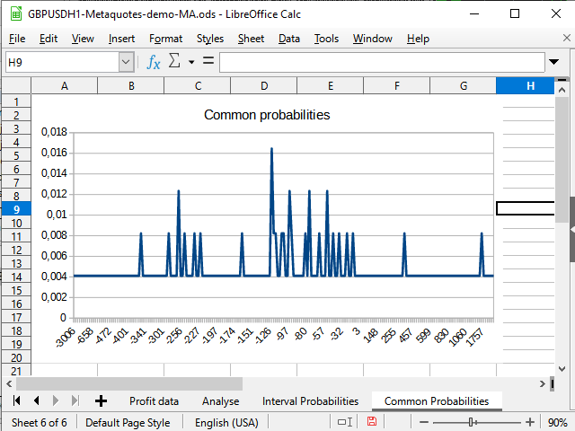
Figure 14. "Immediate" probabilities distribution graph

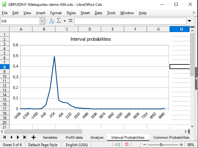
Figure 15. The graph of interval distributions of completed deals' probabilities

Figure 14 demonstrates the negative shift in the probability density. Figure 15 shows a clearly visible peak from -942 to 2154 and a spike (one deal) at 8944.

I believe, the analysis sheet will not cause any particular difficulties (considering everything that has been analyzed).

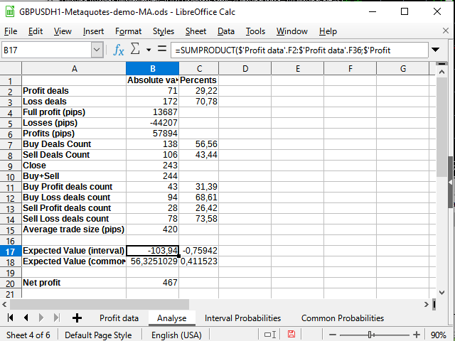
Figure 16. Some statistical calculations

The only new thing here is using the Sumproduct function accepting two intervals as parameters and returning the sum of the products of the members of these intervals (for example, the first row to the first row, the second to the second, and so on). I used this function to calculate the expected payoff. I decided not to apply any more complex integration methods.

The expected payoff is significantly less than the obtained profit and fluctuates around 0 in percentage terms.

Thus, the strategy works but may suffer from very large drawdowns. Probably, it works perfectly during very strong trends (a ~ 9000 pips surge would seem quite interesting, if it were not so lonely), however, the flat will most likely take its toll. The strategy needs serious revision either by introducing pending orders, for example take profits (of about 420-500 pips), or some trend filters. Improvements require additional research.

Running the strategy in the tester

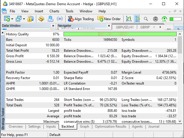
Figure 17. "Examples\Moving Average" EA test results

To be honest, the EA results surprised me. The fact that it opened deals where the table suggested closing them and vice versa may be probably considered normal since its decisions could be based on more or less data (for example, in my table, 25.11.2019 starts at 19:00, while I gave the EA the task to start from the beginning of the day).

I was more surprised by the fact that some deals looked as follows...

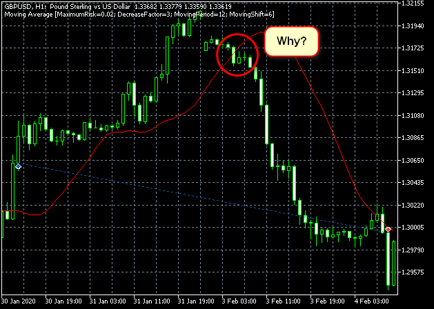
Figure 18. Can my understanding of the algorithm be wrong? Or is something wrong with the tester?

Most likely, I simply did not search well enough and failed to find the reason for such behavior in the algorithm.

The second strange fact was that the EA made 20 more deals than my table suggested. But nevertheless, the results are close to mine, as strange as it may seem.

EA in the tester	Table
Expected payoff — +0.07 (almost 0)	Expected payoff — -0.76 — +0.41 (fluctuates around 0)
Profitable/unprofitable trades — 26.52%/73.48%	Profitable/unprofitable trades — 29.22%/70.78% (considering the difference of 8% in the number of trades, the difference of 3% can be considered insignificant here)

The tester profitability graph and the one found using the table are quite similar: fluctuations around 0 with the difference of about ±500 pips with a spike in February:

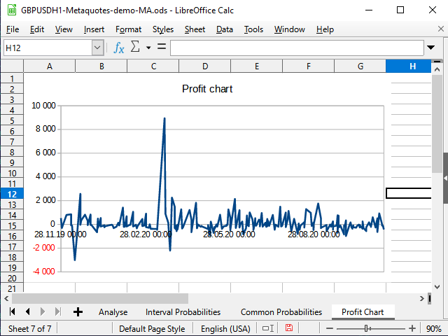
Figure 19. Table profitability graph

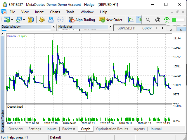
Figure 20. Tester profitability graph

Preparation of the table and tinkering at numbers took about half an hour. Instead for developing an EA, I decided to use a ready-made one. It took about 10 minutes to figure out the algorithm in broad lines. However, there is no need to write a new EA to understand I probably will not use it... Developing an EA is reasonable only if I realize the strategy is worth it. Besides, I prefer manual trading at the moment :-)

Conclusion

I believe, spreadsheets are a very good tool for testing and developing strategies, especially for those having no programming skills, as well as for those willing to create a prototype quickly and convert it into MQL afterwards.

Of course, spreadsheet processor equations sometimes resemble a program code and formatting is less visually clear there.

However, the clarity of spreadsheets, the ability to instantly test new ideas, highlighting affecting cells, diagrams of any kind etc. make spreadsheets an indispensable tool.

If you keep a log of transactions in a table or are able to import it, then using spreadsheet processors allows you to easily improve your strategy and detect mistakes in your trading.