
Using the Kalman Filter for price direction prediction

Introduction
The charts of currency and stock rates always contain price fluctuations, which differ in frequency and amplitude. Our task is to determine the main trends based on these short and long movements. Some traders draw trendlines on the chart, others use indicators. In both cases, our purpose is to separate the true price movement from noise caused by the influence of minor factors that have a short-term effect on the price. In this article I propose using the Kalman filter to separate the major movement from the market noise.
The idea of using digital filters in trading is not new. For example, I have already described the use of low-pass filters. But there is no limit to perfection, so let us consider one more strategy and compare results.
1. Kalman Filter Principle
So, what is the Kalman filter and why is it interesting to us? Here is the definition of the filter from Wikipedia:
Kalman filter is an algorithm that uses a series of measurements observed over time, containing statistical noise and other inaccuracies.
It means that the filter was originally designed to work with noisy data. Also, it is able to work with incomplete data. Another advantage is that it is designed for and applied in dynamic systems; our price chart belongs to such systems.
The filter algorithm works in a two-step process:
- Extrapolation (prediction)
- Update (correction)
1.1. Extrapolation, Prediction of System Values
The first phase of the filter operation algorithm utilizes an underlying model of the process being analyzed. Based on this model, a one-step forward prediction is formed.
![]() (1.1)
(1.1)
Where:
- xk is the extrapolated value of the dynamic system at the k-th step,
- Fk is the state transition model showing the dependence of the current system state on the previous state,
- x^k-1 is the previous state of the system (filter value at the previous step),
- Bk is the control-input model showing the control influence on the system,
- uk is the control vector on the system.
A control effect can be, for example, a news factor. However, in practice the effect is unknown and is omitted, while its influence refers to noise.
Then the system's covariance error is predicted:
![]() (1.2)
(1.2)
Where:
- Pk is the extrapolated covariance matrix of the dynamic system state vector,
- Fk is the state transition model showing the dependence of the current system state on the previous state,
- P^k-1 is the covariance matrix of the state vector updated at the previous step,
- Qk is the covariance noise matrix of the process.
1.2. Update of System Values
The second step of the filter algorithm starts with the measurement of the actual system state zk. The actually measured value of the system state is specified taking into account the true system state and the measurement error. In our case, the measurement error is the effects of noise on the dynamic system.
To this moment, we have two different values that represent the state of a single dynamic process. They include the extrapolated value of the dynamic system calculated at the first step, and the actual measured value. Each of these values with a certain degree of probability characterizes the true state of our process, which, therefore, is somewhere between these two value. So, our goal is to determine the confidence, i.e. the extent, to which this or that value is trusted. Iterations of the Kalman filter's second phase are performed for this purpose.
Using available data, we determine the deviation of the actual system state from the extrapolated value.
![]() (2.1)
(2.1)
Here:
- yk is the deviation of the actual state of the system at the k-th step after extrapolation,
- zk is the actual state of the system at the k-th step,
- Hk is the measurement matrix that displays dependence of the actual system state on the calculated data (often takes a value of one in practice),
- xk is the extrapolated value of the dynamic system at the k-th step.
At the next step, a covariance matrix for the error vector is calculated:
![]() (2.2)
(2.2)
Here:
- Sk is the covariance matrix of the error vector at the k-th step,
- Hk is the measurement matrix that displays dependence of the actual system state on the calculated data,
- Pk is the extrapolated covariance matrix of the dynamic system state vector,
- Rk is the covariance matrix of the measurement noise.
Then the optimal gain is determined. Gain reflects the confidence in the calculated and empirical values.
![]() (2.3)
(2.3)
Here:
- Kk is the matrix of Kalman gain values,
- Pk is the extrapolated covariance matrix of the dynamic system state vector,
- Hk is the measurement matrix that displays dependence of the actual system state on the calculated data,
- Sk is the covariance matrix of the error vector at the k-th step.
Now, we use Kalman gain to update the system state value and the covariance matrix of the state vector estimate.
![]() (2.4)
(2.4)
Where:
- x^k and x^k-1 are updated values at the k-th and k-1 step,
- Kk is the matrix of Kalman gain values,
- yk is the deviation of the actual state of the system at the k-th step after extrapolation.
![]() (2.5)
(2.5)
Where:
- P^k is the updated covariance matrix of the dynamic system state vector,
- I is the identity matrix,
- Kk is the matrix of Kalman gain values,
- Hk is the measurement matrix that displays dependence of the actual system state on the calculated data,
- Pk is the extrapolated covariance matrix of the dynamic system state vector.
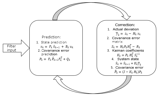
All the above can be summarized as the following scheme
2. Practical Implementation of Kalman Filter
Now, we've got an idea of how the Kalman filter works. Let's move on to its practical implementation. The above matrix representation of filter formulas allows receiving data from several sources. I suggest building a filter at the bar close prices and simplify the matrix representation to a discrete one.
2.1. Initialization of Input Data
Before starting to write the code, let us define input data.
As mentioned above, the basis of the Kalman filter is a dynamic process model, which is used to predict the next state of the process. The filter was initially intended for use with linear systems, in which the current state can be easily defined by applying a coefficient to the previous state. Our case is a little more difficult: our dynamic system is non-linear, and the ratio varies step by step. Moreover, we have no idea about the relationship between neighboring states of the system. The task may seem insoluble. Here is a tricky solution: we will use autoregressive models described in articles [1],[2],[3].
Let's begin. First, we declare the CKalman class and required variables inside this class
class CKalman
  {
private:
//---
   uint              ci_HistoryBars;               //Bars for analysis
   uint              ci_Shift;                     //Shift of autoregression calculation
   string            cs_Symbol;                    //Symbol
   ENUM_TIMEFRAMES   ce_Timeframe;                 //Timeframe
   double            cda_AR[];                     //Autoregression coefficients
   int               ci_IP;                        //Number of autoregression coefficients
   datetime          cdt_LastCalculated;           //Time of LastCalculation;

   bool              cb_AR_Flag;                   //Flag of autoregression calculation
//--- Values of Kalman's filter
   double            cd_X;                         // X
   double            cda_F[];                      // F array
   double            cd_P;                         // P
   double            cd_Q;                         // Q
   double            cd_y;                         // y
   double            cd_S;                         // S
   double            cd_R;                         // R
   double            cd_K;                         // K

public:
                     CKalman(uint bars=6240, uint shift=0, string symbol=NULL, ENUM_TIMEFRAMES period=PERIOD_H1);
                    ~CKalman();
   void              Clear_AR_Flag(void)  {  cb_AR_Flag=false; }
  };
We assign initial values to variables in the class initialization function.
CKalman::CKalman(uint bars, uint shift, string symbol, ENUM_TIMEFRAMES period)
  {
   ci_HistoryBars =  bars;
   cs_Symbol      =  (symbol==NULL ? _Symbol : symbol);
   ce_Timeframe   =  period;
   cb_AR_Flag     =  false;
   ci_Shift       =  shift;
   cd_P           =  1;
   cd_K           =  0.9;
  }
I used an algorithm from the article [1] to create an autoregressive model. Two private functions need to be added to the class for this purpose.
   bool              Autoregression(void);
   bool              LevinsonRecursion(const double &R[],double &A[],double &K[]);
The LevinsonRecursion function is used as is. The Autoregression function has been slightly modified, so let us consider this function in detail. At the beginning of the function we check the availability of history data required for the analysis. If there are not enough historic data, false is returned.
bool CKalman::Autoregression(void)
  {
   //--- check for insufficient data
   if(Bars(cs_Symbol,ce_Timeframe)<(int)ci_HistoryBars)
      return false;
Now, we load the required history data and fill the array of actual state transition model coefficients.
//---
   double   cda_QuotesCenter[];                          //Data to calculate

//--- make all prices available
   double close[];
   int NumTS=CopyClose(cs_Symbol,ce_Timeframe,ci_Shift+1,ci_HistoryBars+1,close)-1;
   if(NumTS<=0)
      return false;
   ArraySetAsSeries(close,true);
   if(ArraySize(cda_QuotesCenter)!=NumTS)
     {
      if(ArrayResize(cda_QuotesCenter,NumTS)<NumTS)
         return false;
     }
   for(int i=0;i<NumTS;i++)
      cda_QuotesCenter[i]=close[i]/close[i+1];           // Calculate coefficients
After the preparatory operations, we determine the number of coefficients of the autoregressive model and calculate their values.
   ci_IP=(int)MathRound(50*MathLog10(NumTS));
   if(ci_IP>NumTS*0.7)
      ci_IP=(int)MathRound(NumTS*0.7);                         // Autoregressive model order

   double cor[],tdat[];
   if(ci_IP<=0 || ArrayResize(cor,ci_IP)<ci_IP || ArrayResize(cda_AR,ci_IP)<ci_IP || ArrayResize(tdat,ci_IP)<ci_IP)
      return false;
   double a=0;
   for(int i=0;i<NumTS;i++)
      a+=cda_QuotesCenter[i]*cda_QuotesCenter[i];
   for(int i=1;i<=ci_IP;i++)
     {
      double c=0;
      for(int k=i;k<NumTS;k++)
         c+=cda_QuotesCenter[k]*cda_QuotesCenter[k-i];
      cor[i-1]=c/a;                                            // Autocorrelation
     }

   if(!LevinsonRecursion(cor,cda_AR,tdat))                     // Levinson-Durbin recursion
      return false;
Now we reduce the sum of the autoregressive coefficients to '1' and set the flag of calculation performance to 'true'.
double sum=0; for(int i=0;i<ci_IP;i++) { sum+=cda_AR[i]; } if(sum==0) return false; double k=1/sum; for(int i=0;i<ci_IP;i++) cda_AR[i]*=k;cb_AR_Flag=true;
Next, we initialize the variables required for the filter. For the calculation noise covariance, we use the root-mean-square value of deviations of Close values for the analyzed period.
cd_R=MathStandardDeviation(close);
To determine the value of the process noise covariance, we first calculate the array of autoregressive model values and find the root-mean-square deviation of the model values.
   double auto_reg[];
   ArrayResize(auto_reg,NumTS-ci_IP);
   for(int i=(NumTS-ci_IP)-2;i>=0;i--)
     {
      auto_reg[i]=0;
      for(int c=0;c<ci_IP;c++)
        {
         auto_reg[i]+=cda_AR[c]*cda_QuotesCenter[i+c];
        }
     }
   cd_Q=MathStandardDeviation(auto_reg);
Then we copy actual state transition coefficients to the cda_F array, from where they can be further used to calculate new coefficients.
   ArrayFree(cda_F);
   if(ArrayResize(cda_F,(ci_IP+1))<=0)
      return false;
   ArrayCopy(cda_F,cda_QuotesCenter,0,NumTS-ci_IP,ci_IP+1);
For the initial value of our system, let us use the arithmetic mean of the last 10 values.
cd_X=MathMean(close,0,10);
2.2. Price Movement Prediction
After we have received all the initial data required for the filter operation, we can proceed to its practical implementation. The first step of Kalman Filter operation is the one-step forward system state prediction. Let us create the Forecast public function in which we will implement functions 1.1. and 1.2.
double Forecast(void);
At the beginning of the function, we check if the regression model has already been calculated. Its calculation function should be called if necessary. EMPTY_VALUE is returned in case of model recalculation error,
double CKalman::Forecast()
  {
   if(!cb_AR_Flag)
     {
      ArrayFree(cda_AR);
      if(Autoregression())
        {
         return EMPTY_VALUE;
        }
     }
After that we calculate the state transition coefficient and save it to the "0" cell of the cda_F array, the values of which are preliminary shifted by one cell.
   Shift(cda_F);
   cda_F[0]=0;
   for(int i=0;i<ci_IP;i++)
      cda_F[0]+=cda_F[i+1]*cda_AR[i];
Then we recalculate the system state and the probability of error.
   cd_X=cd_X*cda_F[0];
   cd_P=MathPow(cda_F[0],2)*cd_P+cd_Q;
The function returns the predicted system state at the end. In our case it is the predicted close price of a new bar.
   return cd_X;
  }
2.3. Correction of the System State
At the next phase, after receiving the actual bar close value, we correct the system state. For this purpose, let's create the public Correction function. In the function parameters, we will pass the actual system state value, i.e. the actual bar closing price.
double Correction(double z);
The theoretical section 1.2. of the given article is implemented in this function. Its full code is available in the attachment. At the end of operation, the function returns the updated (corrected) value of the system state.
3. Practical Demonstration of the Kalman Filter
Let's test how this Kalman filter based class works in practice. Let's create an indicator based on this class. At the opening of a new candlestick, the indicator calls the system update function and then calls the function predicting the close price of the current bar. The class functions are called in a reverse order, because we call the update (correction) function for the previous closed bar and a forecast for the current newly opened bar, whose closing price is yet unknown.
The indicator will have two buffers. The predicted values of the system state will be added to the first buffer, and updated values will be added to the second one. I intentionally use two buffers so that the indicator would not be redrawn and we could see how the system is updated (corrected) at the second filter operation phase. The indicator code is simple and is available in the below attachment. Here is the result of the indicator operation.

Three broken lines are displayed on the chart:
- The black line shows the actual bar closing values
- The red line shows the predicted value
- The blue line is the system state updated by the Kalman filter
As you can see, both lines are close to the actual close prices and show reversal points with good probability. Note that the indicator does not redraw values and the red line is drawn at the opening of the bar when the close price is not yet known.
This chart shows the consistency of this filter and the possibility of creating a trading system using this filter.
4. Creating a Trading Signals Module for the MQL5 Wizard
We see on the above chart that the red system state prediction line is smoother than the black line showing the actual price. The blue line showing the corrected system state is always in between. In other words, the blue line above the red one indicates a bullish trend. Conversely, the blue line below the red one is an indication of a bearish trend. The intersection of the blue and red lines is a trend change signal.
To test this strategy, let's create a module of trading signals for the MQL5 Wizard. The creation of trading signal modules is described in various articles available in this site: [1], [4], [5]. Here, I'll briefly describe points related to the described strategy.
First, we create the CSignalKalman module class, which is inherited from CExpertSignal. Since our strategy is based on the Kalman filter, we need to declare in our class an instance of the CKalman class created above. We declare the CKalman class instance in the module, so it will also be initialized in the module. For that reason, we need to pass initial parameters to the module. That's how the above tasks are implemented in the code:
//+---------------------------------------------------------------------------+
// wizard description start
//+---------------------------------------------------------------------------+
//| Description of the class                                                  |
//| Title=Signals of Kalman's filter design by DNG                            |
//| Type=SignalAdvanced                                                       |
//| Name=Signals of Kalman's filter design by DNG                             |
//| ShortName=Kalman_Filter                                                   |
//| Class=CSignalKalman                                                       |
//| Page=https://www.mql5.com/ru/articles/3886                                |
//| Parameter=TimeFrame,ENUM_TIMEFRAMES,PERIOD_H1,Timeframe                   |
//| Parameter=HistoryBars,uint,3000,Bars in history to analysis               |
//| Parameter=ShiftPeriod,uint,0,Period for shift                             |
//+---------------------------------------------------------------------------+
// wizard description end
//+------------------------------------------------------------------+
//|                                                                  |
//+------------------------------------------------------------------+
class CSignalKalman: public CExpertSignal
  {
private:
   ENUM_TIMEFRAMES   ce_Timeframe;        //Timeframe
   uint              ci_HistoryBars;      //Bars in history to analysis
   uint              ci_ShiftPeriod;      //Period for shift
   CKalman          *Kalman;              //Class of Kalman's filter
   //---
   datetime          cdt_LastCalcIndicators;

   double            cd_forecast;         // Forecast value
   double            cd_corretion;        // Corrected value
   //---
   bool              CalculateIndicators(void);

public:
                     CSignalKalman();
                    ~CSignalKalman();
   //---
   void              TimeFrame(ENUM_TIMEFRAMES value);
   void              HistoryBars(uint value);
   void              ShiftPeriod(uint value);
   //--- method of verification of settings
   virtual bool      ValidationSettings(void);
   //--- method of creating the indicator and timeseries
   virtual bool      InitIndicators(CIndicators *indicators);
   //--- methods of checking if the market models are formed
   virtual int       LongCondition(void);
   virtual int       ShortCondition(void);
  };
In the class initialization function, we assign default values to variables and initialize the Kalman filter class.
CSignalKalman::CSignalKalman(void):    ci_HistoryBars(3000),
                                       ci_ShiftPeriod(0),
                                       cdt_LastCalcIndicators(0)
  {
   ce_Timeframe=m_period;

   if(CheckPointer(m_symbol)!=POINTER_INVALID)
      Kalman=new CKalman(ci_HistoryBars,ci_ShiftPeriod,m_symbol.Name(),ce_Timeframe);
  }
Calculation of the system state using the filter is performed in the CalculateIndicators function. At the beginning of the function we need to check if the filter values have been calculated on the current bar. If the values have already been recalculated, exit the function.
bool CSignalKalman::CalculateIndicators(void)
  {
   //--- Check time of last calculation
   datetime current=(datetime)SeriesInfoInteger(m_symbol.Name(),ce_Timeframe,SERIES_LASTBAR_DATE);
   if(current==cdt_LastCalcIndicators)
      return true;                  // Exit if data already calculated on this bar
Then check the last system state. If it is not defined, reset the autoregressive model calculation flag in the CKalman class—in this case the model will be recalculated during the next call of the class.
   if(cd_corretion==QNaN)
     {
      if(CheckPointer(Kalman)==POINTER_INVALID)
        {
         Kalman=new CKalman(ci_HistoryBars,ci_ShiftPeriod,m_symbol.Name(),ce_Timeframe);
         if(CheckPointer(Kalman)==POINTER_INVALID)
           {
            return false;
           }
        }
      else
         Kalman.Clear_AR_Flag();
     }
At the next step we need to check how many bars have emerged since the previous function call. If the interval is too large, reset the autoregressive model calculation flag.
   int shift=StartIndex();
   int bars=Bars(m_symbol.Name(),ce_Timeframe,current,cdt_LastCalcIndicators);
   if(bars>(int)fmax(ci_ShiftPeriod,1))
     {
      bars=(int)fmax(ci_ShiftPeriod,1);
      Kalman.Clear_AR_Flag();
     }
Then recalculate the system state values for all uncalculated bars.
   double close[];
   if(m_close.GetData(shift,bars+1,close)<=0)
     {
      return false;
     }

   for(uint i=bars;i>0;i--)
     {
      cd_forecast=Kalman.Forecast();
      cd_corretion=Kalman.Correction(close[i]);
     }
After the recalculation, check the system state and save the last function call time. If the operations have successfully completed, the function returns true.
   if(cd_forecast==EMPTY_VALUE || cd_forecast==0 || cd_corretion==EMPTY_VALUE || cd_corretion==0)
      return false;

   cdt_LastCalcIndicators=current;
  //---
   return true;
  }
The structures of the decision-making functions (LongCondition and ShortCondition) are completely identical and use opposite conditions for trade opening. Here is the example of the ShortCondition function code.
First, we start the filter value recalculation function. If the recalculation of values fails, exit the function and return 0.
int CSignalKalman::ShortCondition(void)
  {
   if(!CalculateIndicators())
      return 0;
If the filter values are successfully recalculated, compare the predicted value with the corrected one. If the predicted value is greater than the corrected one, the function returns a weight value. Otherwise 0 is returned.
   int result=0;
   //---
   if(cd_corretion<cd_forecast)
      result=80;
   return result;
  }
The module is built on the "reversal" principle, so we do not implement position closing function.
The code of all functions can be found in the files attached to the article.
5. Expert Advisor Testing
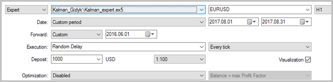
A detailed description of Expert Advisor creation based on the signals module is provided in article [1], so we skip this step. Note that for the testing purposes, the EA is only based on one trading module described above with a static lot and without using a trailing stop.
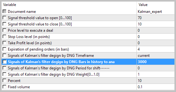
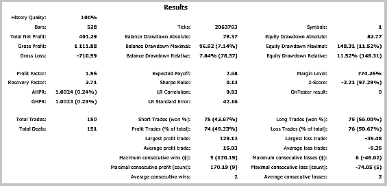
The Expert Advisor was tested using history data of EURUSD for August 2017, with the Н1 timeframe. History data of 3000 bars, i.e. almost 6 months, were used for the calculation of the autoregressive model. The EA was tested without stop loss and take profit to see the clear influence of the Kalman filter on trading.
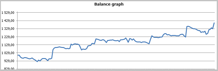
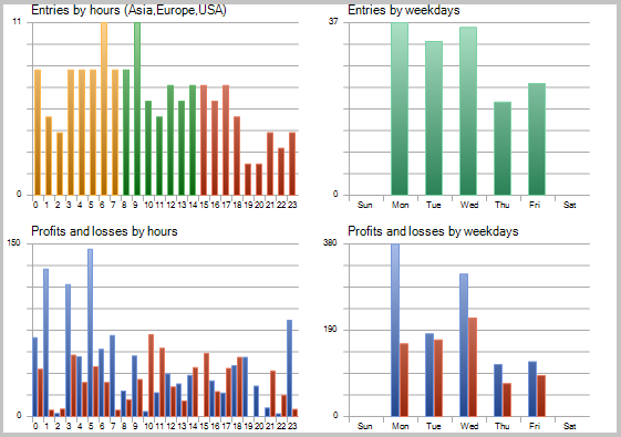
Testing results showed 49.33% of profitable trades. The profits of the highest and average profitable deal exceed the corresponding values of losing trades. In general, the EA testing showed profit for the selected period, and the profit factor was 1.56. Testing screenshots are provided below.
A detailed analysis of trades on the chart reveals the following two weak points of this tactic:
- series of losing deals in flat movements
- late exit from open positions

The same problem areas were also revealed when testing the Expert Advisor using the adaptive market following strategy. Options for resolving these issues were suggested in the mentioned article. However, unlike the previous strategy, the Kalman filter based EA showed a positive result. In my opinion, the strategy proposed and described in this article can become successful if supplemented with an additional filter for determining flat movements. The results might probably be improved by utilizing a time filter. Another option to improve results is to add position exit signals to prevent profits from being lost in case of sharp reverse movements.
Conclusion
We have analyzed the principle of the Kalman filter and have created an indicator and an Expert Advisor on its basis. Testing has shown that this is a promising strategy and has helped reveal a number of bottlenecks that need to be addressed.
Please note that the article only provides general information and an example of creating an Expert Advisor, which in no way is a "Holy Grail" for use in real trading.
I wish everyone a serious approach to trading and profitable trades!
URL Links
- Practical Evaluation of the Adaptive Market Following Method
- Analysis of the Main Characteristics of Time Series
- AR Extrapolation of Price - Indicator for MetaTrader 5
- MQL5 Wizard: How to Create a Module of Trading Signals
- Create Your Own Trading Robot in 6 Steps!
- MQL5 Wizard: New Version
Programs used in the article:
| # |
Name |
Type |
Description |
|---|---|---|---|
| 1 | Kalman.mqh | Class library | Kalman Filter class |
| 2 | SignalKalman.mqh | Class library | A Kalman filter based trading signals module |
| 3 | Kalman_indy.mq5 | Indicator | The Kalman Filter indicator |
| 4 | Kalman_expert.mq5 | EA | An Expert Advisor based on the strategy utilizing the Kalman filter |
| 5 | Kalman_test.zip | Archive | The archive contains the EA testing results obtained by running the EA in the Strategy Tester. |
Translated from Russian by MetaQuotes Ltd.
Original article: https://www.mql5.com/ru/articles/3886
Warning: All rights to these materials are reserved by MetaQuotes Ltd. Copying or reprinting of these materials in whole or in part is prohibited.
This article was written by a user of the site and reflects their personal views. MetaQuotes Ltd is not responsible for the accuracy of the information presented, nor for any consequences resulting from the use of the solutions, strategies or recommendations described.

 Resolving entries into indicators
 R-squared as an estimation of quality of the strategy balance curve
 Comparing different types of moving averages in trading
- Free trading apps
- Over 8,000 signals for copying
- Economic news for exploring financial markets
You agree to website policy and terms of use
The indicator compiled normally. When trying to compile the Expert Advisor, I get the following errors:
'TimeFrame' - unexpected token, probably type is missing? SignalKalman.mqh 153 16
'TimeFrame' - function already defined and has different type SignalKalman.mqh 153 16
'HistoryBars' - unexpected token, probably type is missing? SignalKalman.mqh 166 16
'HistoryBars' - function already defined and has different type SignalKalman.mqh 166 16
'ShiftPeriod' - unexpected token, probably type is missing?SignalKalman.mqh 176 16
'ShiftPeriod' - function already defined and has different type SignalKalman.mqh 176 16
What am I doing wrong?
New MT5 builds require explicitly specifying the type of the returned result of the method. To fix the error, you should add void at the beginning of the specified lines
New MT5 builds require explicitly specifying the type of the returned method result. To fix the error, you should add void to the beginning of the specified lines
Hi Dmitriy. Firstly, congrats for your work!
A question, does the indicator just work in EURUSD? I tried in another pairs and CFDs, the lines are streights and far from the prices.
Awesome for EURUSD
Bad for USDJPY
And BAD for Brasilian Index