R-squared as an estimation of quality of the strategy balance curve

MetaTrader 5 — Trading | 11 December 2017, 12:02

15 528

Introduction

Every trading strategy needs an objective assessment of its effectiveness. A wide range of statistical parameters are used for this. Many of them are easy to calculate and show intuitive metrics. Others are more difficult in construction and interpretation of values. Despite all this diversity, there are very few qualitative metrics for estimating a non-trivial but at the same time obvious value - smoothness of the balance line of the trading system. This article proposes a solution to this problem. Let us consider such a non-trivial measurement, as the coefficient of determination R-squared (R^2), which calculates the qualitative estimation of the most attractive, smooth, rising balance line every trader aspires to.

Of course, the MetaTrader 5 terminal already provides a developed summary report showing the main statistics of the trading system. However, the parameters presented in it are not always sufficient. Fortunately, MetaTrader 5 provides the ability to write custom estimation parameters, which is what we are going to do. Not only will we build the coefficient of determination R^2, but also try to estimate its values, compare it with other optimization criteria, derive regularities followed by the basic statistical estimates.

Criticism of common statistics for trading system evaluation

Every time a trade report is generated or results of trading system backtests are studied, we are presented with several "magic numbers", which can be analyzed to draw conclusions about the quality of the trade. For example, a typical test report in the MetaTrader 5 terminal looks like this:

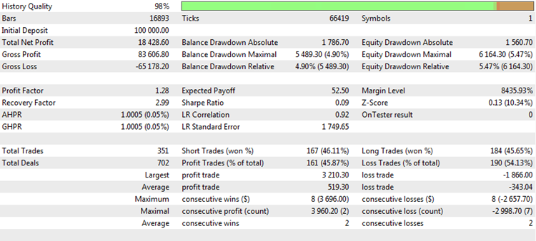
Fig. 1. Backtest result of a trading strategy

It contains a number of interesting statistics or metrics. Let us analyze the most popular of them and objectively consider their strengths and weaknesses.

Total Net Profit. The metric shows the total amount of money that was earned or lost during the testing or trading period. This is one of the most important trading parameters. The primary objective of every trader is to maximize profit. There are various ways to do this, but the final outcome is always one, which is the net profit. Net profit does not always depend on the number of deals and is practically independent of other parameters, although the opposite is not true. Thus, it is invariant in relation to other metrics, and therefore can be used independently of them. However, this measurement has serious drawbacks as well.

First, the net profit is directly dependent on whether capitalization is used or not. When capitalization is used, profit grows non-linearly. Often there is an exponential, explosive growth of the deposit. In this case, the numbers recorded as net profit at the end of testing often reach astronomical values and have nothing to do with reality. If a fixed lot is traded, the deposit increments are more linear, but even in this case the profit depends on the selected volume. For example, if testing, with the result shown in the above table, was performed using a fixed lot with the volume of 0.1 contact, then the obtained profit of $15,757 can be considered a remarkable result. If the deal volume was 1.0 lot, then the testing result is more than modest. This is why the experienced testers prefer setting a lot fixed to 0.1 or 0.01 the Forex market. In this case, the minimum change in the balance is equal to one point of the instrument, which makes the analysis of this characteristic more objective.

Second, the final result depends on the length of the tested period or the duration of the trade history. For example, net profit specified in the table above could have been received in 1 year or in 5 years. And in each case, the same figure means a completely different effectiveness of a strategy.

And third, the gross profit is fixed at the time of the last date. However, there may be a strong drawdown of capital at that moment, whereas it might not have been there a week ago. In other words, this parameter is deeply dependent on the start and end points selected for testing or generating the report.

Profit Factor. This is arguably the most popular statistics for professional traders. While novices want to see only the total profit, professionals find it essential to know the turnover of the invested funds. If the loss of a deal is considered as kind of investment, then Profit Factor shows the marginality of the trading. For example, if only two deals are made, the first one lost $1000 and the second one earned $2000, the Profit Factor of this strategy will be $2000/1000 = 2.0. This is a very good figure. Moreover, Profit Factor neither depends on the testing time span nor on the base lot volume. Therefore, professionals like it so much. However, it has drawbacks as well.

One of them is that the Profit Factor values are highly dependent on the number of deals. If there are only a few deals, obtaining a Profit Factor equal to 2.0 or even 3.0 units is quite possible. On the other hand, if there are numerous deals, then obtaining a Profit Factor of 1.5 units would be a big success.

Expected Payoff. It is a very important characteristic, indicating the Average Deal Return. If the strategy is profitable, the Expected Payoff is positive; losing strategies have a negative value. If the Expected Payoff is comparable to spread or commission costs, the ability of such a strategy to earn on a real account is doubtful. Normally, the Expected Payoff can be positive in the Strategy Tester under ideal execution conditions, and the balance graph can be a smooth ascending line. In live trading, however, the Average Deal Return may turn out slightly worse than the theoretically calculated result due to possible so-called requotes or slippages, which may have a critical impact on the result of the strategy and cause real losses.

It also has its drawbacks. The main one is related to the number of deals too. If there are few deals, obtaining a large Expected Payoff is not a problem. On the other hand, with a large number of deals, the Expected Payoff tends to zero. As it is a linear metric, it cannot be used in strategies implementing money management systems. But professional traders highly regard it and use it in linear systems with a fixed lot, comparing it with the number of deals.

Number of Deals. This is an important parameter that affects most other characteristics explicitly or indirectly. Suppose that a trading system wins in 70% of the cases. At the same time, the absolute values of win and loss are equal, with no other possible outcomes of a deal in the trading tactic. Such a system seems to be outstanding, but what happens it is efficiency is evaluated only based on the last two deals? In 70% of the cases, one of them will be profitable, but the probability of both deals being profitable is only 49%. That is, the total result of two deals will be zero in more than half the cases. Consequently, in half the cases, the statistics will show that the strategy is unable to make money. Its Profit Factor will always be equal to one, Expected Payoff and profit will be zero, other parameters will also indicate zero efficiency.

This is why the number of deals must be sufficiently large. But what is meant by sufficiency? It is generally accepted that any sample should contain at least 37 measurements. This is a magical number in statistics, it marks the lower bound of a parameter's representativeness. Naturally, this amount of deals is not enough to evaluate a trading system. At least 100-10 deals need to be made for the result to be reliable. Moreover, this is also not enough for many professional traders. They design systems that make at least 500-1000 deals and later use these results to consider the possibility of running the system for live trading.

Behavior of common statistical parameters when testing trading systems

The main parameters in the statistics of trading systems have been discussed. Let us see their performance in practice. At the same time, we will focus on their drawbacks to see how the proposed addition in the form of R^2 statistic can help in solving them. To do this, we will use the ready-to-use CImpulse 2.0 EA, which is described in the article "Universal Expert Advisor: Use of Pending Orders". It was chosen for its simplicity and for being optimizable, unlike the experts from the standard MetaTrader 5 package, which is extremely important for the purposes of this article. In addition, a certain code infrastructure will be required, which has already been written for the CStrategy trade engine, so there is no need to do the same job twice. All the source codes for the coefficient of determination are written in such a way that they can easily be used outside CStrategy — for example, in third-party libraries or procedural experts.

Total Net Profit. As already mentioned, the net (or total) profit is the final result of what the trader wants to get. The greater the profit, the better. However, evaluation of a strategy based on its final profit does not always guarantee success. Let us consider the results of the CImpulse 2.0 strategy on the EURUSD pair for the testing period from 2015.01.15 to 2017.10.10:

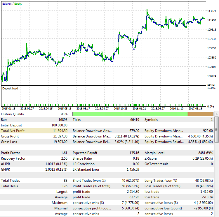
Fig. 2. The CImpulse strategy, EURUSD, 1H, 2015.01.15 - 2017.10.01, PeriodMA: 120, StopPercent: 0.67

The strategy is seen to be showing steady growth of the total profit on this testing interval. It is positive and amounts to 11,894 USD for trading one contract. This is a good result. But let us see what a different scenario looks like, where the final profit is close to the first case:

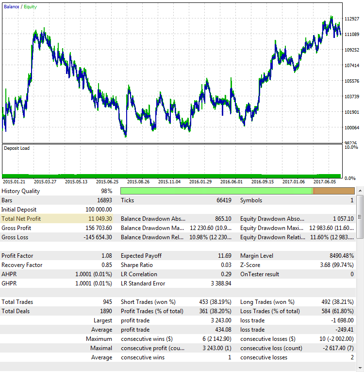
Fig. 3. The CImpulse strategy, EURUSD, 1H, 2015.01.15 - 2017.10.01, PeriodMA: 110, StopPercent: 0.24

Despite the fact that the profit is almost the same in both cases, they look like completely different trading systems. The final profit in the second case also seems random. If the test had ended in the middle of 2015, the profit would have been close to zero.

Here is another unsuccessful run of the strategy, with the final result, however, also very close to the first case:

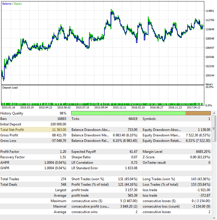
Fig. 4. CImpulse, EURUSD, 1H, 2015.01.15 - 2017.10.01, PeriodMA: 45, StopPercent: 0.44

It is clear from the chart that the main profit was received in the first half of 2015. It is followed by a prolonged period of stagnation. Such a strategy is not a viable option for live trading.

Profit Factor. The Profit Factor metric is much less dependent on the final result. This value depends on each deal and shows the ratio of all funds won to all funds lost. It can be seen that in Fig. 2, Profit Factor is quite high; in Fig. 4, it is lower; and in Fig. 3, it is almost lies on the border between profitable and unprofitable systems. But, nevertheless, Profit Factor is not a universal characteristic that cannot be deceived. Let us examine other examples, where the Profit Factor indications are not so obvious:

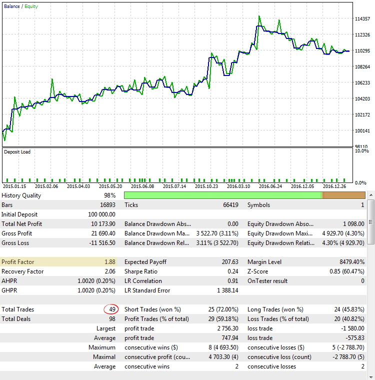
Fig. 5. CImpulse, EURUSD, 1H, 2015.01.15 - 2017.10.01, PeriodMA: 60, StopPercent: 0.82

Fig. 5 shows the result a strategy test run with one of the greatest Profit Factor values. The balance graph looks quite promising, but the statistic obtained is misleading, as the Profit Factor value is overstated due to the very small number of trades.

Let us verify this statement in two ways. The first way: find out the dependence of Profit Factor on the number of trades. This is done by optimizing the CImpulse strategy in the strategy tester using a wide range of parameters:

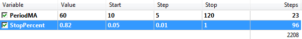
Fig. 6. Optimization of CImpulse using a wide range of parameters

Save the optimization results:

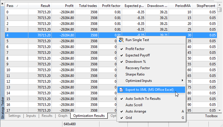
Fig. 7. Exporting optimization results

Now we can build a dependence chart of the Profit Factor value on the number of trades. In Excel, for example, this can be done simply by selecting the corresponding columns and pressing the button for plotting a scatter chart in the Charts tab.

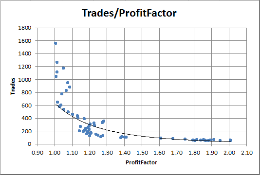
Fig. 8. Dependence of Profit Factor on the number of trades

The chart clearly shows that the runs with a high Profit factor always have very few trades. Conversely, with a large number of trades, Profit Factor is virtually equal to one.

The second way to determine that the ProfitFactor values in this case depend on the number of trades and not the quality of the strategy is related to performing an Out Of Sample test (OOS). By the way, this is one of the most reliable ways to determine the robustness of the obtained results. Robustness is a measure of the stability of a statistical method in estimates. OOS is effective for testing not only ProfitFactor, but other indications as well. For our purposes, the same parameters will be selected, but the time interval will differ — from 2012.01.01 to 2015.01.01:

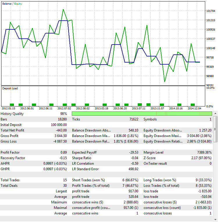
Fig. 9. Testing the strategy out of sample

As it can be seen, the behavior of the strategy turns upside down. It generates loss instead of profit. This is a logical outcome, as the obtained result is almost always random with such a small number of trades. This means that a random win in one time interval is compensated by a loss in another, which is well illustrated by Fig. 9.

Expected Payoff. We will not dwell on this parameter much, because its flaws are similar to those of Profit Factor. Here is the dependence chart of the Expected Payoff on the number of trades:

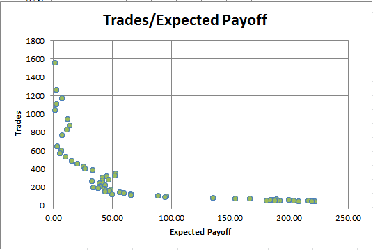
Fig. 10. Dependence of Expected Payoff on the number of trades

It can be seen that the more trades are made, the smaller the Expected Payoff becomes. This dependence is always observed for both profitable and unprofitable strategies. Therefore, Expected Payoff cannot serve as the only criterion for the optimality of a trading strategy.

Requirements for the testing criterion of the trading system

After considering the main criteria of statistical evaluation of a trading system, it has been concluded that the applicability of each criterion is limited. Each of them can be countered with an example where the metric has a good result, while the strategy itself does not.

There are no ideal criteria for determining the robustness of a trading system. But it is possible to formulate the properties that a strong statistical criterion must have.

Independence from the test period duration. Many parameters of a trading strategy depend on how long the testing period is. For example, the greater the tested period for a profitable strategy, the greater the final profit. It depends on duration and recovery factor. It is calculated as the ratio of the total profit to the maximum drawdown. Since the profit depends on the period, the recovery factor also grows with the increase in the testing period. Invariance (independence) relative to the period is necessary to compare the effectiveness of different strategies on different testing periods;
Independence from the testing endpoint. For example, if a strategy "stays afloat" merely by waiting for the losses to pass, the endpoint may have a crucial impact on the final balance. If testing is completed at the time of such "overstaying", the floating loss (equity) become the balance and a significant drawdown is received on the account. The statistic should be protected from such fraud and provide an objective overview of the trading system operation.
Simplicity of interpretation. All parameters of the trading system are quantitative, i.e. each statistic is characterized by a specific figure. This figure must be intuitive. The simpler the interpretation of the obtained value, the more comprehensible the parameter. It is also desirable for the parameter to be within certain bounds, since analysis of large and potentially infinite numbers is often complicated.
Representative results with a small number of deals. This is arguably the most difficult requirement among the characteristics of a good metric. All statistical methods depend on the number of measurements. The more of them, the more stable the obtained statistics. Of course, solving this problem in a small sample completely is impossible. However, it is possible to mitigate the effects caused by the lack of data. For this purpose, let us develop two types of the function for evaluating R squared: one implementation will build this criterion based on the number of available deals. The other one calculates the criterion using the floating profit of the strategy (equity).

Before proceeding directly to the description of the coefficient of determination R^2, let us examine its components in detail. This will help in understanding the purpose of this parameter and the principles it is based on.

Linear Regression

Linear regression is a linear dependence of one variable y from another independent variable x, expressed by the formula y = ax+b. In this formula, а is the multiplier, b is the bias coefficient. In reality, there may be several independent variables, and such model is called a multiple linear regression model. However, we will consider only the simplest case.

Linear dependence can be visualized in the form of a simple graph. Take the daily EURUSD chart from 2017.06.21 to 2017.09.21. This segment is not selected by chance: during this period, a moderate ascending trend was observed on this currency pair. This is how it looks in MetaTrader:

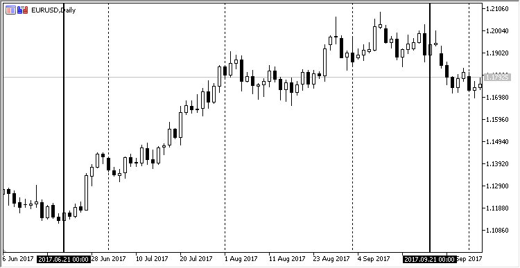
Fig. 11. Dynamics of the EURUSD price from 21.06.2017 to 21.08.2017, daily timeframe

Save these price data and use them to plot a chart, for example, in Excel.

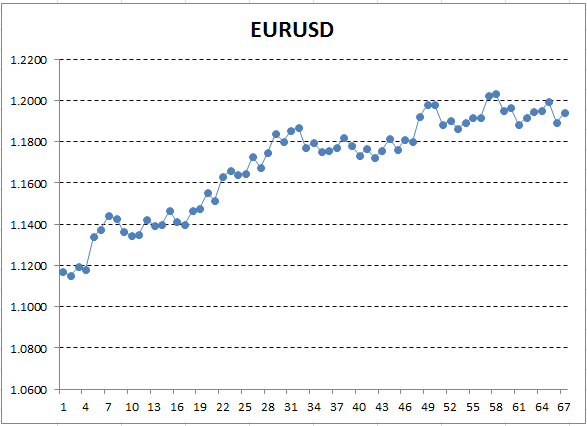
Fig. 12. EURUSD rates (Close price) as a chart in Excel

Here, the Y axis corresponds to the price, and X is the ordinal number of measurement (dates were replaced by ordinal numbers). On the resulting graph, the ascending trend is visible to a naked eye, but we need to obtain a quantitative interpretation of this trend. The simplest way is to draw a straight line, which would fit the examined trend the most accurately. It is called linear regression. For example, the line can be drawn like this:

Fig. 13. Linear regression describing an uptrend, drawn manually

If the graph is fairly smooth, it is possible to draw such a line, that the graph points deviate from it by the minimum distance. And conversely, for a graph with a large amplitude, it is not possible to pick a line that would accurately describe its changes. This is due to the fact that linear regression has only two coefficients. Indeed, the geometry courses taught us that two points are sufficient to plot a line. Due to this, it is not easy to fit a straight line to a "curved" graph. This is a valuable property that will be useful further ahead.

But how to find out how to draw a straight line correctly? Mathematical methods can be used to optimally calculate the linear regression coefficients in such a way that all the available points will have the minimum sum of distances to this line. This is explained on the following chart. Suppose there are 5 arbitrary points and two lines passing through them. From the two lines, it is necessary to select the one with the least sum of distances to the points:

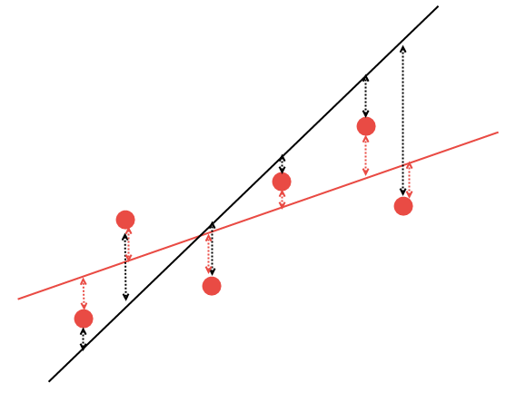
Fig. 14. Selection of the most suitable linear regression

It is clear that, of the two linear regression variants, the red line describes the given data better: points #2 and #6 are significantly closer to the red line than to the black one. The remaining points are approximately equidistant both from the black line and the red one. Mathematically, it is possible to calculate the coordinates of the line that would best describe this regularity. Let us not calculate these coefficients manually and use the ready-to-use AlgLib mathematical library instead.

Correlation

Once the linear regression is calculated, it is necessary to calculate the correlation between this line and the data for which it is calculated. Correlation is statistical relationship of two or more random variables. In this case, the randomness of the variables means that the measurements of these variables are not interdependent. The correlation is measured from -1.0 to +1.0. A value close to zero indicates that the examined variables have no interrelations. The value of +1.0 means a direct dependence, -1.0 shows an inverse dependence. Correlation is calculated by several different formulas. Here, the Pearson's correlation coefficient will be used:

dx and dy in the formula correspond to variances calculated for random variables x and y. Variance is a measure of the variation of the trait. In the most general terms, it can be described as the sum of squares of the distances between the data and the linear regression.

The correlation coefficient of data to their linear regression shows how well the straight line describes these data. If the points of data are located at a great distance from the line, the variance is high and the correlation is low, and vice versa. The correlation is very easy to interpret: a zero value means that there is no interrelation between the regression and data; a value close to one shows a strong direct dependence.

Reports in MetaTrader have a special statistical metric. It is called LR Correlation, and it shows the correlation between the balance curve and linear regression found for that curve. If the balance curve is smooth, the approximation to a straight line will be good. In this case, the LR Correlation coefficient will be close to 1.0, or at least above 0.5. If the balance curve is unstable, then the rises are alternated by falls, and the correlation coefficient tends to zero.

LR Correlation is an interesting parameter. But in statistics, it is not customary to compare the data and the describing regression directly through the correlation coefficient. The reason for this will be discussed in the next section.

Coefficient of determination R^2

Calculation method for the coefficient of determination R^2 is similar to calculation method for LR Correlation. But the final value is additionally squared. It can take values from 0.0 to +1.0. This figure shows the share of the explained values from the total sample. Linear regression serves as an explanatory model. Strictly speaking, the explanatory model does not have to be a linear regression, others can be used as well. However, the R^2 values do not require further processing for a linear regression. In more complex models, the approximation is usually better and the R^2 values must be additionally reduced by special "penalties" for a more adequate estimation.

Let us have a closer look at what the explanatory model shows. To do this, we will perform a small experiment: use the specialized programming language R-Project and generate a random walk, for which the required coefficient will be calculated. Random walk is a process with characteristics quite similar to real financial instruments. To obtain a random walk, it is sufficient to consecutively add several random numbers distributed according to the normal law.

The source code in R with a detailed description of what is being done:

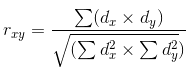
x <- rnorm(1000)            # Generate 1000 random numbers, distributed according to the normal law
                            # Their variance is equal to one, and the expected value is zero
rwalk <- cumsum(x)          # Cumulatively sum these numbers, obtaining a classic random walk graph
plot(rwalk, type="l", col="darkgreen")       # Display the data in the form of a linear graph
rws <- lm(rwalk~c(1:1000))  # Plot the linear model y=a*x+b, where x is the number of measurement, and y is the value of the generated walk vector
title("Line Regression of Random Walk")
abline(rws)                 # Display the resulting linear regression on the chart

The rnorm function returns different data every time, so if you want to repeat this experiment, the graph will have a different look.

The result of the presented code:

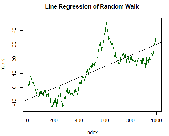
Fig. 15. Random walk and linear regression for it

The resulting chart is similar to that of an arbitrary financial instrument. Its linear regression has been calculated and output as a black line of the chart. At first glance, its description of random walk dynamics is quite mediocre. But we need a quantitative estimation of the linear regression quality. For this purpose, the 'summary' function is used, which outputs the summarized statistics on the regression model:

summary(rws)
Call:
lm(formula = rwalk ~ c(1:1000))

Residuals:
    Min      1Q  Median      3Q     Max 
-16.082  -6.888  -1.593   4.174  30.787 

Coefficients:
             Estimate Std. Error t value Pr(>|t|)    
(Intercept) -8.187185   0.585102  -13.99   <2e-16 ***
c(1:1000)    0.038404   0.001013   37.92   <2e-16 ***
---
Signif. codes:  0 ‘***’ 0.001 ‘**’ 0.01 ‘*’ 0.05 ‘.’ 0.1 ‘ ’ 1

Residual standard error: 9.244 on 998 degrees of freedom
Multiple R-squared:  0.5903,    Adjusted R-squared:  0.5899 
F-statistic:  1438 on 1 and 998 DF,  p-value: < 2.2e-16

Here, one figure is of the most interest — R-squared. This metric indicates a value of 0.5903. Consequently, the linear regression describes 59.03% of all values, and the remaining 41% are left unexplained.

This is a very sensitive indicator that responds well to a smooth, flat line of data. To illustrate this, let us continue the experiment: introduce a stable growth component to the random data. To do this, change the mean value or the expected value by 1/20 of the variance of the initially generated data:

x_trend1 <- x+(sd(x)/20.0)      # Find the standard deviation of values x, divide it by 20.0 and add the obtained value to each value of x
                                # Each such modified value of x will be stored in a new value vector x_trend1
rwalk_t1 <- cumsum(x_trend1)    # Cumulatively sum these numbers, obtaining a shifted random walk graph     
plot(rwalk_t1, type="l", col="darkgreen")        # Display the data as a linear graph
title("Line Regression of Random Walk #2")
rws_t1 <- lm(rwalk_t1~c(1:1000))# Plot the linear model y=a*x+b, where x is the number of measurement, and y is the value of the generated walk vector
abline(rws_t1)                  # Display the resulting linear regression on the chart

The resulting graph is now much closer to a straight line:

Fig. 16. Random walk with positive expected value, equal to 1/20 of its variance

The statistics for it are as follows:

summary(rws_t1)

Call:
lm(formula = rwalk_t1 ~ c(1:1000))

Residuals:
    Min      1Q  Median      3Q     Max 
-16.082  -6.888  -1.593   4.174  30.787 

Coefficients:
             Estimate Std. Error t value Pr(>|t|)    
(Intercept) -8.187185   0.585102  -13.99   <2e-16 ***
c(1:1000)    0.087854   0.001013   86.75   <2e-16 ***
---
Signif. codes:  0 ‘***’ 0.001 ‘**’ 0.01 ‘*’ 0.05 ‘.’ 0.1 ‘ ’ 1

Residual standard error: 9.244 on 998 degrees of freedom
Multiple R-squared:  0.8829,    Adjusted R-squared:  0.8828 
F-statistic:  7526 on 1 and 998 DF,  p-value: < 2.2e-16

It is clear that R-squared is significantly higher and has a value of 0.8829. But let us go for the extra mile and double the determination component of the chart, up to 1/10 of the standard deviation of the initial data. The code to process this is similar to the previous code, but with division by 10.0 and not by 20.0. The new graph is now almost completely resembles a straight line:

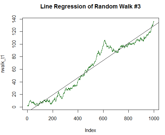
Fig. 17. Random walk with positive expected value, equal to 1/10 of its variance

Calculate its statistics:

Call:
lm(formula = rwalk_t1 ~ c(1:1000))

Residuals:
    Min      1Q  Median      3Q     Max 
-16.082  -6.888  -1.593   4.174  30.787 
4
Coefficients:
             Estimate Std. Error t value Pr(>|t|)    
(Intercept) -8.187185   0.585102  -13.99   <2e-16 ***
c(1:1000)    0.137303   0.001013  135.59   <2e-16 ***
---
Signif. codes:  0 ‘***’ 0.001 ‘**’ 0.01 ‘*’ 0.05 ‘.’ 0.1 ‘ ’ 1

Residual standard error: 9.244 on 998 degrees of freedom
Multiple R-squared:  0.9485,    Adjusted R-squared:  0.9485 
F-statistic: 1.838e+04 on 1 and 998 DF,  p-value: < 2.2e-16

R-squared became even higher and amounted to 0.9485. This graph is very much like the balance dynamics of the desired profitable trading strategy. Let us go for the extra mile again. Increase the expected value up to 1/5 of the standard deviation:

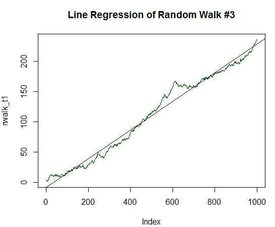
Fig. 18. Random walk with positive expected value, equal to 1/5 of its variance

It has the following statistics:

Call:
lm(formula = rwalk_t1 ~ c(1:1000))

Residuals:
    Min      1Q  Median      3Q     Max 
-16.082  -6.888  -1.593   4.174  30.787 

Coefficients:
             Estimate Std. Error t value Pr(>|t|)    
(Intercept) -8.187185   0.585102  -13.99   <2e-16 ***
c(1:1000)    0.236202   0.001013  233.25   <2e-16 ***
---
Signif. codes:  0 ‘***’ 0.001 ‘**’ 0.01 ‘*’ 0.05 ‘.’ 0.1 ‘ ’ 1

Residual standard error: 9.244 on 998 degrees of freedom
Multiple R-squared:  0.982,     Adjusted R-squared:  0.982 
F-statistic: 5.44e+04 on 1 and 998 DF,  p-value: < 2.2e-16

It is clear that R-squared is now almost equal to one. The chart clearly shows that the random data in the form of the green line almost completely lie on the smooth straight line.

The arcsine theorem and its contribution to the estimation of linear regression

There is a mathematical proof that a random process eventually moves farther away from its original point. It was named the first and second arcsine theorems. They will not be discussed in details, only the corollary of these theorems will be defined.

Based on them, trends in random processes are rather inevitable than unlikely. In other words, there are more random trends in such processes than random fluctuations near the initial point. This is a very important property, which makes a significant contribution to the evaluation of statistical metrics. This is especially evident for the linear regression coefficient (LR Correlation). Trends are better described by linear regression that flats. This is due to the fact that trends contain more movements in one direction, which looks line a smooth line.

If there are more trends in random processes that flats, then LR Correlation will also overestimate its values in general. To see this nontrivial effect, let us try generating 10000 independent random walks with a variance of 1.0 and zero expected value. Let us calculate LR Correlation for each such chart, and then plot a distribution of these values. For these purposes, write a simple test script in R:

sample_r2 <- function(samples = 100, nois = 1000)
{
   lags <- c(1:nois)
   r2 <- 0  # R^2 rating
   lr <- 0  # Line Correlation rating
   for(i in 1:samples)
   {
      white_nois <- rnorm(nois)
      walk <- cumsum(white_nois)
      model <-  lm(walk~lags)
      summary_model <- summary(model)
      r2[i] <- summary_model$r.squared*sign(walk[nois])
      lr[i] <- (summary_model$r.squared^0.5)*sign(walk[nois])
   }
   m <- cbind(r2, lr)
}

The script calculates both LR Correlation and R^2. The difference between them will be seen later. A small addition has been made to the script. The resulting correlation coefficient will be multiplied by the final sign of the synthetic graph. If the final result is less than zero, the correlation will be negative; otherwise it is positive. This is done to easily and quickly separate negative outcomes from positive ones without resorting to other statistics. This is how LR Correlation works in MetaTrader 5, the same principle will be used for R^2.

So, let us plot the distribution of LR Correlation for 10000 independent samples, each of which consists of 1000 measurements:

ms <- sample_r2(10000, nois=1000)
hist(ms[,2], breaks = 30, col="darkgreen", density = 30, main = "Distribution of LR-Correlation")

The resulting graph clearly indicates :correctness of the definition:

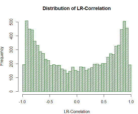
Fig. 19. Distribution of LR-Correlation for 10000 random walks

As seen from the experiment, LR-Correlation values are substantially overestimated in the range of +/- 0.75 - 0.95. This means that LR-Correlation often falsely gives a high positive estimate where it should not.

Now let us consider how R^2 behaves on the same sample:

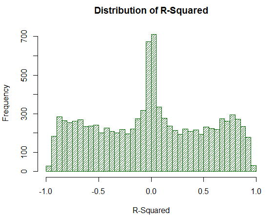
Fig. 20. Distribution of R^2 for 10000 random walks

The R^2 value is not too high, although its distribution is uniform. It is surprising how a simple mathematical action (raising to the power of two) completely negates the undesirable tip effects of the distribution. This is the reason why LR-Correlation can not be analyzed directly — additional mathematical transformation is necessary. Also, note that R^2 moves a significant fraction of the analyzed virtual balances of strategies to a point near zero, while LR-Correlation gives them stable average estimates. This is a positive property.

Collecting the strategy equity

Now that the theory has been studied, it remains to implement R-squared in the MetaTrader terminal. Of course, we could go for the easy way and calculate it for the deals in history. However, an additional improvement will be introduced. As mentioned before, any statistical parameter must be resistant to a small number of deals. Unfortunately, R-squared can unreasonably inflate its value if there are only a few deals on the account, like any other statistic. In order to avoid this, calculate it based on the values of equity — floating profit. The idea behind this is that if the EA makes only 20 deals per year, it is very difficult to estimate its efficiency. Its result is most likely random. But if the balance of this EA is measured at a specified periodicity (for example, once an hour), there will be a fair amount of points for plotting the statistic. In this case, there will be more than 6000 measurements.

In addition, such measurement counteracts systems that do not fix their floating loss, thus hiding it. Drawdown by equity is present, but not by balance. A statistic calculated based on balance does not warn about occurring problems. However, a metric calculated with consideration of the floating profit/loss reflects the objective situation on the account.

The equity of the strategy will be collected in an unconventional way. This is because the collection of these values requires two main points to be taken into account:

Frequency of statistics collection
Determination of events, receiving which requires the equity to be checked.

For example, an Expert Advisor works only by timer, on the H1 timeframe. It is tested in the "Opening prices only" mode. Therefore, the data for this EA cannot be collected more than once an hour, and screening of these data can be performed only when the OnTimer event is raised. The most effective solution is simply to use the power of the CStrategy engine. The fact is that CStrategy collects all events into a single event handler, and it monitors the necessary timeframe automatically. Thus, the optima solution is to write a special agent strategy, which calculates all the required statistics. It will be created by the CManagerList strategy manager. The class will only add its agent to the list of strategies, which will monitor the changes on the account.

The source code of this agent is provided below:

//+------------------------------------------------------------------+
//|                                                UsingTrailing.mqh |
//|                                 Copyright 2017, Vasiliy Sokolov. |
//|                                             https://www.mql5.com |
//+------------------------------------------------------------------+
#property copyright "Copyright 2017, Vasiliy Sokolov."
#property link      "https://www.mql5.com"
#include "TimeSeries.mqh"
#include "Strategy.mqh"
//+------------------------------------------------------------------+
//| Integrated to the portfolio of strategies as an expert and       |
//| records the portfolio equity                                     |
//+------------------------------------------------------------------+
class CEquityListener : public CStrategy
{
private:
   //-- Recording frequency
   CTimeSeries       m_equity_list;
   double            m_prev_equity;
public:
                     CEquityListener(void);
   virtual void      OnEvent(const MarketEvent& event);
   void              GetEquityArray(double &array[]);
};
//+------------------------------------------------------------------+
//| Setting the default frequency                                    |
//+------------------------------------------------------------------+
CEquityListener::CEquityListener(void) : m_prev_equity(EMPTY_VALUE)
{
}
//+------------------------------------------------------------------+
//| Collects the portfolio equity, monitoring all possible           |
//| events                                                           |
//+------------------------------------------------------------------+
void CEquityListener::OnEvent(const MarketEvent &event)
{
   if(!IsTrackEvents(event))
      return;
   double equity = AccountInfoDouble(ACCOUNT_EQUITY);
   if(equity != m_prev_equity)
   {
      m_equity_list.Add(TimeCurrent(), equity);
      m_prev_equity = equity;
   }
}
//+------------------------------------------------------------------+
//| Returns the equity as an array of type double                    |
//+------------------------------------------------------------------+
void CEquityListener::GetEquityArray(double &array[])
{
   m_equity_list.ToDoubleArray(0, array);
}

The agent itself consists of two methods: redefined OnEvent and a method for returning the equity values. Here, the main interest is on the CTimeSeries class, which appears in CStrategy for the first time. It is a simple table, with the data added in the format: date, value, column number. All stored values are sorted by time. The required date is accessed via binary search, which substantially speeds up the work with the collection. The OnEvent method checks if the current event is the opening of a new bar, and if so, simply stores the new equity value.

R^2 reacts to a situation where there are no deals for a long time. At such times, the unchanged equity values will be recorded. The equity graph forms a so-called "ladder". To prevent this, the method compares the value with the previous value. If the values match, the record is skipped. Thus, only the changes in equity fall into the list.

Let us integrate this class to the CStrategy engine. Integration will be performed from above, at the level of CStrategyList. This module is suitable for calculation of custom statistics. There can be several custom statistics. Therefore, an enumeration listing all possible statistic types is introduced:

//+------------------------------------------------------------------+
//| Determines the type of custom criterion calculated after         |
//| optimization.                                                    |
//+------------------------------------------------------------------+
enum ENUM_CUSTOM_TYPE
  {
   CUSTOM_NONE,                     // Custom criterion is not calculated
   CUSTOM_R2_BALANCE,               // R^2 based on the strategy balance
   CUSTOM_R2_EQUITY,                // R^2 based on the strategy equity
  };

The enumeration above shows that the custom optimization criterion has three types: R-squared based on the result of trades, R-squared based on the equity data and no calculation of statistics.

Add the ability to configure the type of custom calculation. To do this, supply the CStrategyList class with additional SetCustomOptimaze* methods:

//+------------------------------------------------------------------+
//| Sets R^2 as the optimization criterion. The coefficient is       |
//| calculated for the trades made.                                  |
//+------------------------------------------------------------------+  
void CStrategyList::SetCustomOptimizeR2Balance(ENUM_CORR_TYPE corr_type)
{
   m_custom_type = CUSTOM_R2_BALANCE;
   m_corr_type = corr_type;
}
//+------------------------------------------------------------------+
//| Sets R^2 as the optimization criterion. The coefficient is       |
//| calculated based on the recorded equity.                         |
//+------------------------------------------------------------------+  
void CStrategyList::SetCustomOptimizeR2Equity(ENUM_CORR_TYPE corr_type)
{
   m_custom_type = CUSTOM_R2_EQUITY;
   m_corr_type = corr_type;
}

Each of these methods sets the value of its internal variable of ENUM_CUSTOM_TYPE to m_custom_type and the second parameter, equal to the correlation type ENUM_CORR_TYPE:

//+------------------------------------------------------------------+
//| Correlation type                                                 |
//+------------------------------------------------------------------+
enum ENUM_CORR_TYPE
  {
   CORR_PEARSON,     // Pearson's correlation
   CORR_SPEARMAN     // Spearman's Rank-Order correlation
  };

This additional parameters must be mentioned separately. The fact is that R^2 is none other but the correlation between the graph and its linear model. However, the correlation type itself may differ. Use the AlgLib mathematical library. It supports two methods for calculating the correlation: Pearson's and Spearman's. Pearson's formula is classic and well-suited to homogeneous, normally distributed data. Spearman's Rank-Order correlation is more resistant to price spikes, which are often observed on the market. Therefore, our calculation will allow working with each variant of calculating R^2.

Now that all data are prepared, proceed to the calculation of R^2. It is moved to separate functions:

//+------------------------------------------------------------------+
//| Returns the R^2 estimate based on the strategy balance           |
//+------------------------------------------------------------------+
double CustomR2Balance(ENUM_CORR_TYPE corr_type = CORR_PEARSON);
//+------------------------------------------------------------------+
//| Returns the R^2 estimate based on the strategy equity            |
//| The values of equity are passed as the 'equity' array            |
//+------------------------------------------------------------------+
double CustomR2Equity(double& equity[], ENUM_CORR_TYPE corr_type = CORR_PEARSON);

They will be located in a separate file named RSquare.mqh. The calculation is arranged in the form of functions, so that users would be able to easily and quickly include this calculation mode in their project. In this case, there is no need to use CStrategy. For example, to calculate R^2 in your expert, simply redefine the OnTester system function:

double OnTester()
{
   return CustomR2Balance();
}

When it is necessary to calculate the strategy equity, however, users who do not employ CStrategy will have to do it themselves.

The last thing that needs to be done in CStrategyList is to define the OnTester method:

//+------------------------------------------------------------------+
//| Adds monitoring of equity                                        |
//+------------------------------------------------------------------+
double CStrategyList::OnTester(void)
{
   switch(m_custom_type)
   {
      case CUSTOM_NONE:
         return 0.0;
      case CUSTOM_R2_BALANCE:
         return CustomR2Balance(m_corr_type);
      case CUSTOM_R2_EQUITY:
      {
         double equity[];
         m_equity_exp.GetEquityArray(equity);
         return CustomR2Equity(equity, m_corr_type);
      }
   }
   return 0.0;
}

Now consider the implementation of functions CustomR2Equity and CustomR2Balance.

Calculating the coefficient of determination R^2 using AlgLib

The coefficient of determination R^2 is implemented using AlgLib — a cross-platform library of numerical analysis. It helps calculate various statistical criteria, from simple to the most advanced ones.

Here are the steps for calculating the coefficient.

Get the values of equity and convert them into matrix M[x, y], where x is the number of measurement, y is the equity value.
For the obtained matrix, calculate the a and b coefficients of the linear regression equation.
Generate the linear regression values for each X and put them in the array.
Find the correlation coefficient of linear regression and the equity values using one of the two correlation formulas.
Calculate R^2 and its sign.
Return the normalized value of R^2 to the calling function.

These steps are performed by the CustomR2Equity function. Its source code is presented below:

//+------------------------------------------------------------------+
//| Returns the R^2 estimate based on the strategy equity            |
//| The values of equity are passed as the 'equity' array            |
//+------------------------------------------------------------------+
double CustomR2Equity(double& equity[], ENUM_CORR_TYPE corr_type = CORR_PEARSON)
{
   int total = ArraySize(equity);
   if(total == 0)
      return 0.0;
   //-- Fill the matrix: Y - equity value, X - ordinal number of the value
   CMatrixDouble xy(total, 2);
   for(int i = 0; i < total; i++)
   {
      xy[i].Set(0, i);
      xy[i].Set(1, equity[i]);
   }
   //-- Find coefficients a and b of the linear model y = a*x + b;
   int retcode = 0;
   double a, b;
   CLinReg::LRLine(xy, total, retcode, a, b);
   //-- Generate the linear regression values for each X;
   double estimate[];
   ArrayResize(estimate, total);
   for(int x = 0; x < total; x++)
      estimate[x] = x*a+b;
   //-- Find the coefficient of correlation of values with their linear regression
   double corr = 0.0;
   if(corr_type == CORR_PEARSON)
      corr = CAlglib::PearsonCorr2(equity, estimate);
   else
      corr = CAlglib::SpearmanCorr2(equity, estimate);
   //-- Find R^2 and its sign
   double r2 = MathPow(corr, 2.0);
   int sign = 1;
   if(equity[0] > equity[total-1])
      sign = -1;
   r2 *= sign;
   //-- Return the R^2 estimate normalized to within hundredths
   return NormalizeDouble(r2,2);
}

This code refers to three statistical methods: CAlgLib::LRLine, CAlglib::PearsonCorr2 and CAlglib::SpearmanCorr2. The main one is CAlgLib::LRLine, which directly calculates the linear regression coefficients.

Now let us describe the second function for calculating R^2: CustomR2Balance. As the name implies, this function calculates the value based on the deals made. All its work lies in forming an array of the double type, which contains the dynamics of balance, by iterating over all deals in history.

//+------------------------------------------------------------------+
//| Returns the R^2 estimate based on the strategy balance           |
//+------------------------------------------------------------------+
double CustomR2Balance(ENUM_CORR_TYPE corr_type = CORR_PEARSON)
{
   HistorySelect(0, TimeCurrent());
   double deals_equity[];
   double sum_profit = 0.0;
   int current = 0;
   int total = HistoryDealsTotal();
   for(int i = 0; i < total; i++)
   {
      ulong ticket = HistoryDealGetTicket(i);
      double profit = HistoryDealGetDouble(ticket, DEAL_PROFIT);
      if(profit == 0.0)
         continue;
      if(ArraySize(deals_equity) <= current)
         ArrayResize(deals_equity, current+16);
      sum_profit += profit;
      deals_equity[current] = sum_profit;
      current++;
   }
   ArrayResize(deals_equity, current);
   return CustomR2Equity(deals_equity, corr_type);
}

Once the array is formed, it is passed to the CustomR2Equity function mentioned earlier. In fact, the CustomR2Equity function is universal. It calculates the R^2 value for any data contained in the equity[] array, whether it is the balance dynamics or the value of the floating profit.

The last step is a small modification in the code of the CImpulse EA, namely, the override of the OnTester system event:

//+------------------------------------------------------------------+
//| Tester event                                                     |
//+------------------------------------------------------------------+
double OnTester()
{
   Manager.SetCustomOptimizeR2Balance(CORR_PEARSON);
   return Manager.OnTester();
}

This function sets the type of the custom parameter, and then returns its value.

Now we can see the calculated coefficient in action. Once the CImpulse strategy backtest starts, the parameter will appear in the report:

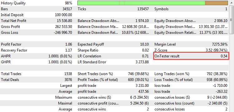
Fig. 21. The value of R^2 as a custom optimization criterion

Using the R-squared parameter in practice

Now that R-squared is built-in as a custom optimization criterion, it is time to try it out in practice. This is done by optimizing CImpulse on the М15 timeframe of the EURUSD currency pair. Save the received optimization result to an Excel file, and then use the obtained statistics to compare several runs selected according to different criteria.

The complete list of optimization parameters is provided below:

Symbol: EURUSD
Timeframe: H1
Period: 2015.01.03 - 2017.10.10

The range of the EA parameters is listed in the table:

Parameter	Start	Step	Stop Sign	Number of steps
PeriodMA	15	5	200	38
StopPercent	0.1	0.05	1.0	19

After the optimization, an optimization cloud was obtained, consisting of 722 variants:

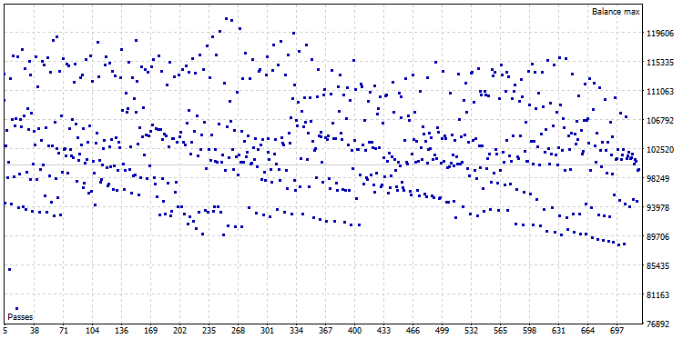
Fig. 22. Optimization cloud of CImpulse, symbol - EURUSD, timeframe - H1

Select the run with the maximum profit and display its balance graph:

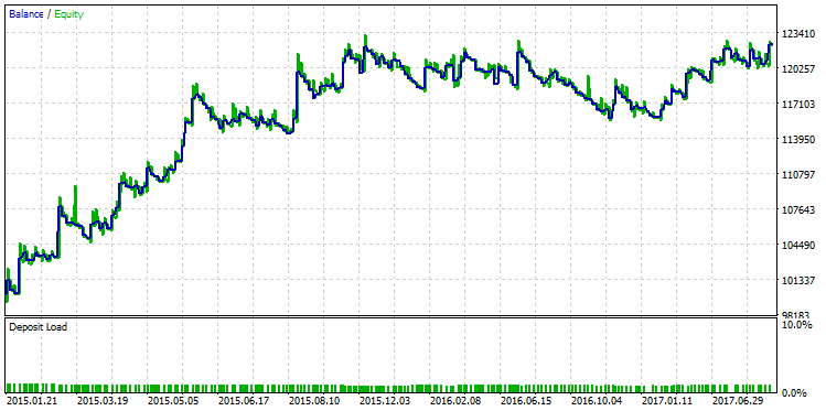
Fig. 23. Balance graph of the strategy selected according to the criterion of the maximum profit

Now find the best run according to the R-square parameter. For this, compare the optimization runs in the XML file. If Microsoft Excel is installed on the computer, the file will be opened in it automatically. The work will involve sorting and filters. Select the table title and press the button of the same name (Home -> Sort & Filter -> Filter). This allows customizing the display of columns. Sort the runs according to the custom optimization criterion:

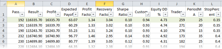
Fig. 24. Optimization runs in Microsoft Excel, sorted by R-squared

The first row in the table will have the best R-squared value of the entire sample. In the figure above, it is marked in green. This set of parameters in the strategy tester gives a balance graph that looks as follows:

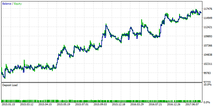
Fig. 25. Balance graph of a strategy selected according to the criterion of the maximum R-squared value

The qualitative difference between these two balance graphs is visible to the naked eye. While the test run with the maximum profit "broke down" in December 2015, the other variant with the maximum R^2 continued its steady growth.

Often R^2 depends on the number of deals, and may usually overestimate its values on small samples. In this respect, R-squared correlates with Profit Factor. On certain strategy types, a high value of Profit Factor and a high value of R^2 go together. However, this is not always the case. As an illustration, select a counter-example from the sample, demonstrating the difference between R^2 and Profit Factor. The figure below shows a strategy run having one of the highest Profit Factor values equal to 2.98:

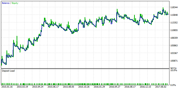
Fig. 26. Test run of a strategy with Profit Factor equal to 2.98

The graph shows that, even though the strategy shows a steady growth, the quality of the strategy balance curve is still lower than the one with the maximum R-squared.

Advantages and limitations of use

Each statistical metric has its pros and cons. R-squared is no exception in this regard. The table below presents its flaws and solutions that can mitigate them:

Drawbacks	The solution
Depends on the number of deals. Overestimates the values with a small number of deals.	Calculation of the R^2 value based on equity of the strategy partially solves this problem.
Correlates with existing metrics of strategy effectiveness, particularly with Profit Factor and Net profit of the strategy.	The correlation is not 100%. Depending on the features of the strategy, R-squared may not correlate with any other metric at all or correlate weakly.
Computation requires complex mathematical calculations.	The algorithm is implemented using the AlgLib library, which is delegated all the complexity.
Applicable exclusively for estimation of linear processes or systems trading with a fixed lot.	Do not apply to trading systems that use a capitalization system (money management).

Let us describe the problem of applying R^2 to nonlinear systems (for example, a trading strategy with a dynamic lot) in more detail.

The primary objective of every trader is the maximization of profit. A necessary condition for this is the use of various capitalization systems. Capitalization system is the transformation of a linear process into a nonlinear one (for example, into an exponential process). But such a transformation renders most of the statistical parameters meaningless. For example, the "final profit" parameter is meaningless for capitalized systems, since even a slight shift in the time interval testing or changing a strategy parameter by a hundredth of a percent can change the final result by tens or even hundreds of times.

Other parameters of the strategy lose their meaning as well, such as Profit Factor, Expected Payoff, the maximum profit/loss, etc. In this sense, R-squared is no exception either. Created for linear estimation of the balance curve smoothness, it becomes powerless in evaluation of nonlinear processes. Therefore, any strategy should be tested in a linear form, and only after that a capitalization system should be added to the selected option. It is better to evaluate nonlinear systems using special statistical metrics (for example, GHPR) or to calculate the yield in annual percentages.

Conclusion

The standard statistical parameters for evaluating trading systems have known drawbacks, which must be taken into account.
Among the standard metrics in MetaTrader 5, only LR Correlation is designed to estimate the smoothness of the strategy balance curve. However, its values are often overestimated.
R-squared is one of the few metrics that calculate the smoothness of both the balance curve and the floating profit curve of the strategy. At the same time, R-squared is free from the disadvantages of LR Correlation.
The AlgLib mathematical library is used in calculation of R-squared. The calculation itself has many modifications and is thoroughly described in the corresponding example.
The custom optimization criterion can be built into an Expert Advisor so that all experts can calculate this metric automatically without their participation. Instructions on how to do this are provided in the example of integrating R-squared into the CStrategy trading engine.
A similar integration method can be used for calculating additional data required in calculation of custom statistics. For R-squared, such data are the data on floating profit of the strategy (equity). Recording of the floating profit dynamics is performed by the CStrategy trading engine.
The coefficient of determination allows selecting strategies with a growth of the balance/equity. In this case, the process of selection based on other parameters may miss such variants.
R-squared has its downsides, like any other statistical metric, which must be taken into account when working with this value.

Thus, it is safe to say that the coefficient of determination R-squared is an important addition to the existing set of the MetaTrader 5 testing metrics. It allows estimating the smoothness of a strategy's balance curve, which is a nontrivial indicator on its own. R-squared is easy to use: its values are bound to the range of -1.0 to +1.0, signaling about a negative trend in the strategy balance (values close to -1.0), no trend (values close to 0.0) and a positive trend (values tending to +1.0). Thanks to all these properties, reliability and simplicity, R-squared can be recommended for use in building a profitable trading system.

Translated from Russian by MetaQuotes Ltd.
Original article: https://www.mql5.com/ru/articles/2358

Attached files |

Download ZIP

UnExpert.zip (114.84 KB)

Warning: All rights to these materials are reserved by MetaQuotes Ltd. Copying or reprinting of these materials in whole or in part is prohibited.