
Statistical Estimations

Introduction
Nowadys, you can often meet articles and publications written on subjects connected with econometrics, forecasting of price series, choosing and estimating adequacy of a model, etc. But in most cases, reasoning is based on assumption, that a reader is acquainted with the methods of math statistics and can easily estimate statistical parameters of an analyzed sequence.
Estimation of statistical parameters of a sequence is very important, since most of mathematical models and methods are based on different assumptions. For example, normality of distribution law or dispersion value, or other parameters. Thus, when analyzing and forecasting of time series we need a simple and convenient tool that allows quickly and clearly estimating the main statistical parameters. In this article, we're going to try to create such a tool.
The article shortly describes the simplest statistical parameters of a random sequence and several methods of its visual analysis. It offers the implementation of these methods in MQL5 and the methods of visualization of the result of calculations using the Gnuplot application. By no means has this article pretended to be a manual or a reference; that is why it may contain certain familiarities accepted regarding the terminology and definitions.
Analyzing Parameters on a Sample
Suppose that there is a stationary process existing endlessly in time, which can be represented as a sequence of discrete samples. Let's call this sequence of samples as the general population. A part of samples selected from the general population will be called a sampling from the general population or a sampling of N samples. In addition to it, suppose that no true parameters are known to us, so we're going to estimate them on the basis of a finite sampling.
Avoiding Outliers
Before starting the statistical estimation of parameters, we should note that the accuracy of estimation may be insufficient if the sampling contains gross errors (outliers). There is a huge influence of outliers on the accuracy of estimations if the sampling has a small volume. Outliers are the values that abnormally diverge from the middle of distribution. Such deviations can be caused by different hardly probable events and errors appeared while gathering statistical data and forming the sequence.
It is hard to make a decision whether to filter outliers or not, since in most cases it is impossible to clearly detect whether a value is an outlier or belongs to the analyzed process. So if outliers are detected and there's a decision to filter them, then a question arises - what should we do with those error values? The most logical variant is excluding from the sampling, what may increase the accuracy of estimation of statistical characteristics; but you should be careful with excluding outliers from sampling when working with time sequences
To have a possibility of excluding outliers from a sampling or at least detecting them, let's implement the algorithm described in the book "Statistics for Traders" written by S.V. Bulashev.
According to this algorithm, we need to calculate five values of estimation of the center of distribution:
- Median;
- Center of 50% interquartile range (midquartile range, MQR);
- Arithmetical mean of entire sampling;
- Arithmetical mean on the 50% interquartile range (interquartile mean, IQM);
- Center of range (midrange) - determined as the average value of the maximum and minimum value in a sampling.
Then the results of estimation of the center of distribution are sorted in ascending order; and then the average value or the third one in order is chosen as the center of distribution Xcen. Thus, the chosen estimation appears to be minimally affected by outliers.
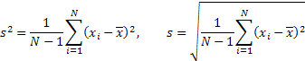
Further, using the obtained estimation of the center of distribution Xcen, let's calculate the standard deviation s, the excess K and the rate of censoring according to the empirical formula:
![]()
where N is the number of samples in the sampling (volume of sampling).
Then the values that lie outside the range:
![]()
will be counted as outliers, thus they should be excluded from the sampling.
This method is described in details in the "Statistics for Traders" book, so let's go straight to implementation of the algorithm. The algorithm that allows detecting and excluding outliers is implemented in the erremove() function.
Below you can find the script written for testing this function.
//----------------------------------------------------------------------------
//                                                                erremove.mq5
//                                   Copyright 2011, MetaQuotes Software Corp.
//                                                         https://www.mql5.com
//----------------------------------------------------------------------------
#property copyright "Copyright 2011, MetaQuotes Software Corp."
#property link      "https://www.mql5.com"
#property version   "1.00"

#import "shell32.dll"
bool ShellExecuteW(int hwnd,string lpOperation,string lpFile,
                  string lpParameters,string lpDirectory,int nShowCmd);
#import
//----------------------------------------------------------------------------
// Script program start function
//----------------------------------------------------------------------------
void OnStart()
  {
  int i;
  double dat[100];
  double y[];

  srand(1);
  for(i=0;i<ArraySize(dat);i++)dat[i]=rand()/16000.0;

  dat[25]=3;           // Make Error !!!

  erremove(dat,y,1);

  }
//----------------------------------------------------------------------------
int erremove(const double &x[],double &y[],int visual=1)
  {
  int i,m,n;
  double a[],b[5];
  double dcen,kurt,sum2,sum4,gs,v,max,min;

  if(!ArrayIsDynamic(y))                           // Error
    {
    Print("Function erremove() error!");
    return(-1);
    }
  n=ArraySize(x);
  if(n<4)                                          // Error
    {
    Print("Function erremove() error!");
    return(-1);
    }
  ArrayResize(a,n);
  ArrayCopy(a,x);
  ArraySort(a);
  b[0]=(a[0]+a[n-1])/2.0;                          // Midrange
  m=(n-1)/2;
  b[1]=a[m];                                       // Median
  if((n&0x01)==0)b[1]=(b[1]+a[m+1])/2.0;
  m=n/4;
  b[2]=(a[m]+a[n-m-1])/2.0;                        // Midquartile range
  b[3]=0;
  for(i=m;i<n-m;i++)b[3]+=a[i];                    // Interquartile mean(IQM)
  b[3]=b[3]/(n-2*m);
  b[4]=0;
  for(i=0;i<n;i++)b[4]+=a[i];                      // Mean
  b[4]=b[4]/n;
  ArraySort(b);
  dcen=b[2];                                       // Distribution center
  sum2=0; sum4=0;
  for(i=0;i<n;i++)
    {
    a[i]=a[i]-dcen;
    v=a[i]*a[i];
    sum2+=v;
    sum4+=v*v;
    }
  if(sum2<1.e-150)kurt=1.0;
  kurt=((n*n-2*n+3)*sum4/sum2/sum2-(6.0*n-9.0)/n)*(n-1.0)/(n-2.0)/(n-3.0); // Kurtosis
  if(kurt<1.0)kurt=1.0;
  gs=(1.55+0.8*MathLog10((double)n/10.0)*MathSqrt(kurt-1))*MathSqrt(sum2/(n-1));
  max=dcen+gs;
  min=dcen-gs;
  m=0;
  for(i=0;i<n;i++)if(x[i]<=max&&x[i]>=min)a[m++]=x[i];
  ArrayResize(y,m);
  ArrayCopy(y,a,0,0,m);

  if(visual==1)vis(x,dcen,min,max,n-m);

  return(n-m);
  }
//----------------------------------------------------------------------------
void vis(const double &x[],double dcen,double min,double max,int numerr)
  {
  int i;
  double d,yma,ymi;
  string str;

  yma=x[0];ymi=x[0];
  for(i=0;i<ArraySize(x);i++)
    {
    if(yma<x[i])yma=x[i];
    if(ymi>x[i])ymi=x[i];
    }
  if(yma<max)yma=max;
  if(ymi>min)ymi=min;
  d=(yma-ymi)/20.0;
  yma+=d;ymi-=d;
  str="unset key\n";
  str+="set title 'Sequence and error levels (number of errors = "+
        (string)numerr+")' font ',10'\n";
  str+="set yrange ["+(string)ymi+":"+(string)yma+"]\n";
  str+="set xrange [0:"+(string)ArraySize(x)+"]\n";
  str+="plot "+(string)dcen+" lt rgb 'green',";
  str+=(string)min+ " lt rgb 'red',";
  str+=(string)max+ " lt rgb 'red',";
  str+="'-' with line lt rgb 'dark-blue'\n";
  for(i=0;i<ArraySize(x);i++)str+=(string)x[i]+"\n";
  str+="e\n";
  if(!saveScript(str)){Print("Create script file error");return;}
  if(!grPlot())Print("ShellExecuteW() error");
  }
//----------------------------------------------------------------------------
bool grPlot()
  {
  string pnam,param;

  pnam="GNUPlot\\binary\\wgnuplot.exe";
  param="-p MQL5\\Files\\gplot.txt";
  return(ShellExecuteW(NULL,"open",pnam,param,NULL,1));
  }
//----------------------------------------------------------------------------
bool saveScript(string scr1="",string scr2="")
  {
  int fhandle;

  fhandle=FileOpen("gplot.txt",FILE_WRITE|FILE_TXT|FILE_ANSI);
  if(fhandle==INVALID_HANDLE)return(false);
  FileWriteString(fhandle,"set terminal windows enhanced size 560,420 font 8\n");
  FileWriteString(fhandle,scr1);
  if(scr2!="")FileWriteString(fhandle,scr2);
  FileClose(fhandle);
  return(true);
  }
//----------------------------------------------------------------------------
Let's take a detailed look at the erremove() function. As the first parameter of the function we pass the address of the array x[], where the values of the analyzed sampling are stored; the sampling volume must be no less than four elements. It is supposed that the size of the x[] array is equal to the sampling size, that's why the N value of volume of the sampling is not passed. Data located in the x[] array is not changed as a result of execution of the function.
The next parameter is the address of the y[] array. In case of successful execution of the function, this array will contain the input sequence with outliers excluded. Size of the y[] array is less than the size of the x[] array by the number of values excluded from the sampling. The y[] array must be declared as a dynamic one, otherwise it will be impossible to change its size in the body of the function.
The last (optional) parameter is the flag responsible for the visualization of the calculation results. If its value is equal to one (default value), then before the end of execution of the function the chart displaying the following information will be drawn in a separate window: the input sequence, the line of center of distribution and the limits of range, values outside of which will be considers as outliers.
The method of drawing charts will be described later. In case of successful execution, the function returns the number of values excluded from the sampling; in case of an error, it returns -1. If no error values (outliers) are discovered, the function will return 0 and the sequence in the y[] array will be the same as in x[].
In the beginning of the function, the information is copied from the x[] to the a[] array, then it is sorted in ascending order, and then five estimations of the center of distribution are made.
The middle of range (midrange) is determined as the sum of extreme values of the sorted array a[] divided by two.
The median is calculated for odd volumes of the sampling N as following:
![]()
and for even volumes of the sampling:
![]()
Considering that indexes of the sorted array a[] start from zero, we get:
m=(n-1)/2;
median=a[m];
if((n&0x01)==0)b[1]=(median+a[m+1])/2.0;
The middle of the 50% interquartile range (midquartile range, MQR):
![]()
where M=N/4 (integer division).
For the sorted array a[] we get:
m=n/4;
MQR=(a[m]+a[n-m-1])/2.0;               // Midquartile range
Arithmetical means of the 50% interquartile range (interquartile mean, IQM). 25% of samples are cut from both sides of the sampling, and the remaining 50% are used for calculation of the arithmetical mean:
![]()
where M=N/4 (integer division).
m=n/4; IQM=0;
for(i=m;i<n-m;i++)IQM+=a[i];
IQM=IQM/(n-2*m);                       // Interquartile mean(IQM)
The arithmetical mean (mean) is determined for the entire sampling.
Each of the determined values is written to the b[] array, and then the array is sorted in ascending order. An element value of the b[2] array is chosen as the center of the distribution. Further, using this value, we will calculate the unbiased estimations of the arithmetical mean and the coefficient of excess; the algorithm of calculation will be described later.
The obtained estimations are used for calculation of the coefficient of censoration and limits of the range for detecting outliers (the expressions are shown above). In the end, the sequence with excluded outliers is formed in the y[] array, and the vis() functions is called for drawing the graph. Let's take a short look at the method of visualization used in this article.
Visualization
To display the results of calculation, I use the freeware application gnuplot intended for making various 2D and 3D graphs. Gnuplot has the possibility of displaying charts on the screen (in a separate window) or writing them to a file in different graphic formats. The commands of plotting charts can be executed from a preliminary prepared text file. The official web page of the gnuplot project is - gnuplot.sourceforge.net. The application is multi-platform, and it is distributed both as the source code files and as binary files compiled for a certain platform.
The examples written for this article were tested under Windows XP SP3 and the 4.2.2 version of gnuplot. The gp442win32.zip file can be downloaded at http://sourceforge.net/projects/gnuplot/files/gnuplot/4.4.2/. I haven't tested the examples with other versions and builds of gnuplot.
Once you download the gp442win32.zip archive, unzip it. As a result, the \gnuplot folder is created, it contains the application, the help file, documentation and examples. To interact with applications, put the entire \gnuplot folder to the root folder of your MetaTrader 5 client terminal.

Figure 1. Placement of the folder \gnuplot
Once the folder is moved, you can change the operability of the gnuplot application. To do it, execute the file \gnuplot\binary\wgnuplot.exe, and then, as the "gnuplot>" command prompt appears, type the "plot sin(x)" command. As a result, a window with the sin(x) function drawn in it should appear. Also you can try the examples included in the application delivery; to do it, choose the File\Demos item and select the file \gnuplot\demo\all.dem.
Now as you start the erremove.mq5 script, the graph demonstrated in the figure 2 will be draw in a separate window:

Figure 2. The graph that is drawn using the erremove.mq5 script.
Further in the article, we are going to talk little about some feature of using gnuplot, since the information about the program and its controls can be easily found in the documentation, which is delivered together with it, and at various websites, such as http://gnuplot.ikir.ru/.
The examples of programs written for this article use a simplest method of interaction with gnuplot for drawing the charts. At first, the text file gplot.txt is created; it contains the gnuplot commands and information to be displayed. Then the wgnuplot.exe application is started with the name of that file passed as an argument in the command line. The wgnuplot.exe application is called using the ShellExecuteW() function imported from the system library shell32.dll; it's the reason why the import of external dlls must be allowed in the client terminal.
The given version of gnuplot allows drawing charts in a separate window for two types of terminals: wxt and windows. The wxt terminal uses the algorithms of antialiasing for drawing of charts, what allows obtaining a higher quality picture comparing to the windows terminal. However, the windows terminal was used for writing the examples for this article. The reason is when working with the windows terminal, the system process created as a result of the "wgnuplot.exe -p MQL5\\Files\\gplot.txt" call and opening of a graph window is automatically killed as the window is closed.
If you choose the wxt terminal, then when you close the chart window, the system process wgnuplot.exe will not be shut down automatically. Thus, if you use the wxt terminal and call wgnuplot.exe for many times as described above, multiple processes without any signs of activity may accumulate in the system. Using the "wgnuplot.exe -p MQL5\\Files\\gplot.txt" call and the windows terminal, you can avoid opening of unwanted additional window and appearing of unclosed system processes.
The window, where the chart is displayed, is interactive and it processes the mouse click and keyboard events. To get the information about default hotkeys, run wgnuplot.exe, choose a type of terminal using the "set terminal windows" command and plot any chart, for example using the "plot sin(x)" command. If the chart window is active (in focus), then you'll see a tip displayed in the text window of wgnuplot.exe as soon as you press the "h" button.
Estimation of Parameters
After the short acquaintance with the method of chart drawing, let's return to the estimation of parameters of the general population on the basis of its finite sampling. Supposing that no statistical parameters of the general population are known, we are going to use only unbiased estimations of these parameters.
The estimation of mathematical expectation or the sampling mean can be considered as the main parameter that determines the distribution of a sequence. The sampling mean is calculated using the following formula:
![]()
where N is the number of samples in the sampling.
The mean value is an estimation of the center of distribution and it is used for calculation of other parameters connected with central moments, what makes this parameter especially important. In addition to the mean value, we will use the estimation of dispersion (dispersion, variance), the standard deviation, the coefficient of skewness (skewness) and the coefficient of excess (kurtosis) as statistical parameters.
![]()
where m are central moments.
Central moments are numeric characteristics of distribution of a general population.
The second, third and fourth selective central moments are determined by the following expressions:
![]()
But those values are unbiased. Here we should mention k-Statistic and h-Statistic. Under certain conditions they allow obtaining unbiased estimations of central moments, so they can be used for calculation of unbiased estimations of dispersion, standard deviation, skewness and kurtosis.
Note that the calculation of the fourth moment in the k and h estimations is performed in different ways. It results in obtaining different expressions for the estimation of kurtosis when using k or h. For example, in Microsoft Excel the excess is calculated using the formula that corresponds to the use of k-estimations, and in the "Statistics for Traders" book, the unbiased estimation of kurtosis is done using the h-estimations.
Let's choose the h-estimations, and then by substituting them instead of 'm' in previously given expression, we will calculate the necessary parameters.
Dispersion and Standard Deviation:
Skewness:
![]()
Kurtosis:
![]()
The coefficient of excess (kurtosis) calculated according to the given expression for the sequence with normal distribution law is equal to 3.
You should pay attention that the value obtained by subtracting 3 from the calculated value is often used as the kurtosis value; thus the obtained value is normalized relatively to the normal distribution law. In the first case, this coefficient is called kurtosis; in the second case, it is called "excess kurtosis".
The calculation of parameters according to the given expression is performed in the dStat() function:
struct statParam
  {
  double mean;
  double median;
  double var;
  double stdev;
  double skew;
  double kurt;
  };
//----------------------------------------------------------------------------
int dStat(const double &x[],statParam &sP)
  {
  int i,m,n;
  double a,b,sum2,sum3,sum4,y[];

  ZeroMemory(sP);                                      // Reset sP
  n=ArraySize(x);
  if(n<4)                                             // Error
    {
    Print("Function dStat() error!");
    return(-1);
    }
  sP.kurt=1.0;
  ArrayResize(y,n);
  ArrayCopy(y,x);
  ArraySort(y);
  m=(n-1)/2;
  sP.median=y[m];                                     // Median
  if((n&0x01)==0)sP.median=(sP.median+y[m+1])/2.0;
  sP.mean=0;
  for(i=0;i<n;i++)sP.mean+=x[i];
  sP.mean/=n;                                         // Mean
  sum2=0;sum3=0;sum4=0;
  for(i=0;i<n;i++)
    {
    a=x[i]-sP.mean;
    b=a*a;sum2+=b;
    b=b*a;sum3+=b;
    b=b*a;sum4+=b;
    }
  if(sum2<1.e-150)return(1);
  sP.var=sum2/(n-1);                                  // Variance
  sP.stdev=MathSqrt(sP.var);                           // Standard deviation
  sP.skew=n*sum3/(n-2)/sum2/sP.stdev;                 // Skewness
  sP.kurt=((n*n-2*n+3)*sum4/sum2/sum2-(6.0*n-9.0)/n)*
                              (n-1.0)/(n-2.0)/(n-3.0); // Kurtosis

  return(1);
When dStat() is called, the address of the x[] array is passed to the function. It contains the initial data and the link to the statParam structure, which will contain calculated values of the parameters. In case of an error occurring when there are less than four elements in the array, the function returns -1.
Histogram
In addition to the parameters calculated in the dStat() function, the law of distribution of the general population is of a big interest for us. To visually estimate the distribution law on the finite sampling, we can draw a histogram. When drawing the histogram, the range of values of the sampling is divided into several similar sections. And then the number of elements in each section is calculated (group frequencies).
Further, a bar diagram is drawn on the basis of group frequencies. It is called a histogram. After normalizing to the range width, the histogram will represent an empiric density of distribution of a random value. Let's use the empiric expression described in the "Statistics for Traders" for determining an optimal number of sections for drawing the histogram:
![]()
where L is the required number of sections, N is the volume of sampling and e is the kurtosis.
Below you can find the dHist(), which determines the number of sections, calculates the number of elements in each of them and normalizes obtained group frequencies.
struct statParam
  {
  double mean;
  double median;
  double var;
  double stdev;
  double skew;
  double kurt;
  };
//----------------------------------------------------------------------------
int dHist(const double &x[],double &histo[],const statParam &sp)
  {
  int i,k,n,nbar;
  double a[],max,s,xmin;

  if(!ArrayIsDynamic(histo))                           // Error
    {
    Print("Function dHist() error!");
    return(-1);
    }
  n=ArraySize(x);
  if(n<4)                                             // Error
    {
    Print("Function dHist() error!");
    return(-1);
    }
  nbar=(sp.kurt+1.5)*MathPow(n,0.4)/6.0;
  if((nbar&0x01)==0)nbar--; if(nbar<5)nbar=5;          // Number of bars
  ArrayResize(a,n);
  ArrayCopy(a,x);
  max=0.0;
  for(i=0;i<n;i++)
    {
    a[i]=(a[i]-sp.mean)/sp.stdev;                     // Normalization
    if(MathAbs(a[i])>max)max=MathAbs(a[i]);
    }
  xmin=-max;
  s=2.0*max*n/nbar;
  ArrayResize(histo,nbar+2);
  ArrayInitialize(histo,0.0);
  histo[0]=0.0;histo[nbar+1]=0.0;
  for(i=0;i<n;i++)
    {
    k=(a[i]-xmin)/max/2.0*nbar;
    if(k>(nbar-1))k=nbar-1;
    histo[k+1]++;
    }
  for(i=0;i<nbar;i++)histo[i+1]/=s;

  return(1);
  }
The address of the x[] array is passed to the function. it contains the initial sequence. The content of the array is not changed as a result of execution of the function. The next parameters is the link to the histo[] dynamic array, where the calculated values will be stored. The number of elements of that array will correspond to the number of sections used for the calculation plus two elements.
One element containing zero value is added to the beginning and to the end of the histo[] array. The last parameter is the address of the statParam structure that should contain the previously calculated values of the parameters stored in it. In case the histo[] array passed to the function is not a dynamic array or the input array x[] contains less than four elements, the function stops its execution and returns -1.
Once you've drawn a histogram of obtained values, you can visually estimate whether the sampling corresponds to the normal law of distribution. For a more visual graphical representation of the correspondence to the normal law of distribution, we can draw a graph with the scale of normal probability (Normal Probability Plot) in addition to the histogram.
Normal Probability Plot
The main idea of drawing such a graph is the X axis should be strained so that the displayed values of a sequence with normal distribution lie on the same line. In this way, the normality hypothesis can be checked graphically. You can find more detailed information about such type of graphs here: "Normal probability plot" or "e-Handbook of Statistical Methods".
To calculate values required for drawing the graph of normal probability, the function dRankit() shown below is used.
struct statParam
  {
  double mean;
  double median;
  double var;
  double stdev;
  double skew;
  double kurt;
  };
//----------------------------------------------------------------------------
int dRankit(const double &x[],double &resp[],double &xscale[],const statParam &sp)
  {
  int i,n;
  double np;

  if(!ArrayIsDynamic(resp)||!ArrayIsDynamic(xscale))    // Error
    {
    Print("Function dHist() error!");
    return(-1);
    }
  n=ArraySize(x);
  if(n<4)                                            // Error
    {
    Print("Function dHist() error!");
    return(-1);
    }
  ArrayResize(resp,n);
  ArrayCopy(resp,x);
  ArraySort(resp);
  for(i=0;i<n;i++)resp[i]=(resp[i]-sp.mean)/sp.stdev;
  ArrayResize(xscale,n);
  xscale[n-1]=MathPow(0.5,1.0/n);
  xscale[0]=1-xscale[n-1];
  np=n+0.365;
  for(i=1;i<(n-1);i++)xscale[i]=(i+1-0.3175)/np;
  for(i=0;i<n;i++)xscale[i]=ltqnorm(xscale[i]);

  return(1);
  }
//----------------------------------------------------------------------------

double A1 = -3.969683028665376e+01, A2 =  2.209460984245205e+02,
       A3 = -2.759285104469687e+02, A4 =  1.383577518672690e+02,
       A5 = -3.066479806614716e+01, A6 =  2.506628277459239e+00;
double B1 = -5.447609879822406e+01, B2 =  1.615858368580409e+02,
       B3 = -1.556989798598866e+02, B4 =  6.680131188771972e+01,
       B5 = -1.328068155288572e+01;
double C1 = -7.784894002430293e-03, C2 = -3.223964580411365e-01,
       C3 = -2.400758277161838e+00, C4 = -2.549732539343734e+00,
       C5 =  4.374664141464968e+00, C6 =  2.938163982698783e+00;
double D1 =  7.784695709041462e-03, D2 =  3.224671290700398e-01,
       D3 =  2.445134137142996e+00, D4 =  3.754408661907416e+00;
//----------------------------------------------------------------------------
double ltqnorm(double p)
  {
  int s=1;
  double r,x,q=0;

  if(p<=0||p>=1){Print("Function ltqnorm() error!");return(0);}
  if((p>=0.02425)&&(p<=0.97575))    // Rational approximation for central region
    {
    q=p-0.5; r=q*q;
    x=(((((A1*r+A2)*r+A3)*r+A4)*r+A5)*r+A6)*q/(((((B1*r+B2)*r+B3)*r+B4)*r+B5)*r+1);
    return(x);
    }
  if(p<0.02425)                    // Rational approximation for lower region
    {
    q=sqrt(-2*log(p));
    s=1;
    }
  else      //if(p>0.97575)          // Rational approximation for upper region
    {
    q = sqrt(-2*log(1-p));
    s=-1;
    }
  x=s*(((((C1*q+C2)*q+C3)*q+C4)*q+C5)*q+C6)/((((D1*q+D2)*q+D3)*q+D4)*q+1);
  return(x);
  }
The address of the x[] array is inputted to the function. The array contains the initial sequence. The next parameters are references to the output arrays resp[] and xscale[]. After the execution of the function, the values used for drawing of the chart on the X and Y axes respectively are written to the arrays. Then the address of the statParam structure is passed to the function. It should contain previously calculated values of the statistical parameters of the input sequence. In case of an error, the function returns -1.
When forming values for the X axis, the function ltqnorm() is called. It calculates the reverse integral function of normal distribution. The algorithm that is used for calculation is taken from "An algorithm for computing the inverse normal cumulative distribution function".
Four Charts
Previously I mentioned the dStat() function where the values of the statistical parameters are calculated. Let's briefly repeat their meaning.
Dispersion (variance) – the mean value of squares of deviation of a random value from its mathematical expectation (average value). The parameter that shows how big is the deviation of a random value from its center of distribution. The more the value of this parameter is, the more is the deviation.
Standard deviation – since the dispersion is measured as the square of a random value, the standard deviation is often used as a more obvious characteristics of dispersion. It is equal to the square root of the dispersion.
Skewness – if we draw a curve of distribution of a random value, the skewness will show how asymmetrical is the curve of probability density relatively to the center of distribution. If the skewness value is greater than zero, the curve of probability density has a steep left slope and a flat right slope. If the skewness value is negative, then the left slope is flat and the right one is steep. When the curve of probability density is symmetric to the center of distribution, the skewness is equal to zero.
The coefficient of excess (kurtosis) – it describes the sharpness of a peak of the curve of probability density and the steepness of slopes of the distribution tails. The sharper is the curve peak near the center of distribution, the greater is the value of the kurtosis.
Despite the fact that mentioned statistical parameters describe a sequence in details, often you can characterize a sequence in an easier way - on the basis of result of estimations represented in a graphical form. For example, an ordinary graph of a sequence can greatly complete a view obtained when analyzing the statistical parameters.
Previously in the article, I have mentioned the dHist() and dRankit() functions that allow preparing data for drawing a histogram or a chart with the scale of normal probability. Displaying the histogram and the graph of normal distribution together with the ordinary graph on the same sheet, allows you determining main features of the analyzed sequence visually.
Those three listed charts should be supplemented with another one - the chart with the current values of the sequence on the Y axis and its previous values on the X axis. Such a chart is called a "Lag Plot". If there is a strong correlation between adjacent indications, values of a sampling will stretch in a straight line. And if there is no correlation between adjacent indications, for example, when analyzing a random sequence, then values will be dispersed all over the chart.
For a quick estimation of an initial sampling, I suggest to draw four charts on a single sheet and to display the calculated values of the statistical parameter on it. This is not a new idea; you can read about using the analysis of four mentioned charts here: "4-Plot".
In the end of the article, there is the "Files" section containing the script s4plot.mq5, which draws those four charts on a single sheet. The dat[] array is created within the OnStart() function of the script. It contains the initial sequence. Then the dStat(), dHist() and dRankit() functions are called consequently for calculation of data required for drawing of the charts. The vis4plot() function is called next. It creates a text file with the gnuplot commands on the basis of the calculated data, and then it calls the application for drawing the charts in a separate window.
There is no point is showing the entire code of the script in article, since the dStat(), dHist() and dRankit() were described previously, the vis4plot() function, which creates a sequence of gnuplot commands, doesn't have any significant peculiarities, and description of the gnuplot commands goes out of bounds of the article subject. In addition to that, you can use another method for drawing the charts instead of the gnuplot application.
So let's shown only a part of the s4plot.mq5 - its OnStart() function.
//----------------------------------------------------------------------------
// Script program start function
//----------------------------------------------------------------------------
void OnStart()
  {
  int i;
  double dat[128],histo[],rankit[],xrankit[];
  statParam sp;

  MathSrand(1);
  for(i=0;i<ArraySize(dat);i++) dat[i]=MathRand();

  if(dStat(dat,sp)==-1)return;
  if(dHist(dat,histo,sp)==-1)return;
  if(dRankit(dat,rankit,xrankit,sp)==-1)return;

  vis4plot(dat,histo,rankit,xrankit,sp,6);
  }
In this example, a random sequence is used for filling the dat[] array with initial data using the MathRand() function. The script execution should result in following:

Figure 3. Four charts. Script s4plot.mq5
You should pay attention to the last parameter of the vis4plot() function. It is responsible for the format of outputted numeric values. In this example, the values are outputted with six decimal places. This parameter is the same as the one that determines the format in the DoubleToString() function.
If values of the input sequence are too small or too big, you can use the scientific format for a more obvious displaying. To do it, set that parameter to -5, for example. The -5 value is set on default for the vis4plot() function.
To demonstrate the obviousness of the method of four charts for displaying of peculiarities of a sequence, we need a generator of such sequences.
Generator of a Pseudo-Random Sequence
The class RNDXor128 is intended for generating pseudo-random sequences.
Below, there is the source code of the include file describing that class.
//-----------------------------------------------------------------------------------
//                                                                      RNDXor128.mqh
//                                                                      2011, victorg
//                                                                https://www.mql5.com
//-----------------------------------------------------------------------------------
#property copyright "2011, victorg"
#property link      "https://www.mql5.com"

#include <Object.mqh>
//-----------------------------------------------------------------------------------
// Generation of pseudo-random sequences. The Xorshift RNG algorithm
// (George Marsaglia) with the 2**128 period of initial sequence is used.
//          uint rand_xor128()
//            {
//            static uint x=123456789,y=362436069,z=521288629,w=88675123;
//            uint t=(x^(x<<11));x=y;y=z;z=w;
//            return(w=(w^(w>>19))^(t^(t>>8)));
//            }
// Methods:
//  Rand()      - even distribution withing the range [0,UINT_MAX=4294967295].
//  Rand_01()   - even distribution within the range [0,1].
//  Rand_Norm() - normal distribution with zero mean and dispersion one.
//  Rand_Exp()  - exponential distribution with the parameter 1.0.
//  Rand_Laplace() - Laplace distribution with the parameter 1.0
//  Reset()     - resetting of all basic values to initial state.
//  SRand()     - setting new basic values of the generator.
//-----------------------------------------------------------------------------------
#define xor32  xx=xx^(xx<<13);xx=xx^(xx>>17);xx=xx^(xx<<5)
#define xor128 t=(x^(x<<11));x=y;y=z;z=w;w=(w^(w>>19))^(t^(t>>8))
#define inidat x=123456789;y=362436069;z=521288629;w=88675123;xx=2463534242

class RNDXor128:public CObject
  {
protected:
  uint      x,y,z,w,xx,t;
  uint      UINT_half;
public:
            RNDXor128()       {UINT_half=UINT_MAX>>1;inidat;};
  double    Rand()            {xor128;return((double)w);};
  int       Rand(double& a[],int n)
                              {int i;if(n<1)return(-1);
                               if(ArraySize(a)<n)return(-2);
                               for(i=0;i<n;i++){xor128;a[i]=(double)w;}
                               return(0);};
  double    Rand_01()         {xor128;return((double)w/UINT_MAX);};
  int       Rand_01(double& a[],int n)
                              {int i;if(n<1)return(-1);
                               if(ArraySize(a)<n)return(-2);
                               for(i=0;i<n;i++){xor128;a[i]=(double)w/UINT_MAX;}
                               return(0);};
  double    Rand_Norm()       {double v1,v2,s,sln;static double ra;static uint b=0;
                               if(b==w){b=0;return(ra);}
                               do{
                                 xor128;v1=(double)w/UINT_half-1.0;
                                 xor128;v2=(double)w/UINT_half-1.0;
                                 s=v1*v1+v2*v2;
                                 }
                               while(s>=1.0||s==0.0);
                               sln=MathLog(s);sln=MathSqrt((-sln-sln)/s);
                               ra=v2*sln;b=w;
                               return(v1*sln);};
  int       Rand_Norm(double& a[],int n)
                              {int i;if(n<1)return(-1);
                               if(ArraySize(a)<n)return(-2);
                               for(i=0;i<n;i++)a[i]=Rand_Norm();
                               return(0);};
  double    Rand_Exp()        {xor128;if(w==0)return(DBL_MAX);
                               return(-MathLog((double)w/UINT_MAX));};
  int       Rand_Exp(double& a[],int n)
                              {int i;if(n<1)return(-1);
                               if(ArraySize(a)<n)return(-2);
                               for(i=0;i<n;i++)a[i]=Rand_Exp();
                               return(0);};
  double    Rand_Laplace()    {double a;xor128;
                              a=(double)w/UINT_half;
                              if(w>UINT_half)
                                {a=2.0-a;
                                if(a==0.0)return(-DBL_MAX);
                                return(MathLog(a));}
                              else
                                {if(a==0.0)return(DBL_MAX);
                                return(-MathLog(a));}};
  int       Rand_Laplace(double& a[],int n)
                              {int i;if(n<1)return(-1);
                               if(ArraySize(a)<n)return(-2);
                               for(i=0;i<n;i++)a[i]=Rand_Laplace();
                               return(0);};
  void      Reset()           {inidat;};
  void      SRand(uint seed)  {int i;if(seed!=0)xx=seed;
                               for(i=0;i<16;i++){xor32;}
                               xor32;x=xx;xor32;y=xx;
                               xor32;z=xx;xor32;w=xx;
                               for(i=0;i<16;i++){xor128;}};
  int       SRand(uint xs,uint ys,uint zs,uint ws)
                              {int i;if(xs==0&&ys==0&&zs==0&&ws==0)return(-1);
                               x=xs;y=ys;z=zs;w=ws;
                               for(i=0;i<16;i++){xor128;}
                               return(0);};
  };
//-----------------------------------------------------------------------------------
The algorithm used for generating a random sequence is described in details in the article "Xorshift RNGs" by George Marsaglia (see the xorshift.zip at the end of the article). Methods of the RNDXor128 class are described in the RNDXor128.mqh file. Using this class, you can get sequences with even, normal or exponential distribution or with Laplace distribution (double exponential).
You should pay attention to the fact, that when an instance of the RNDXor128 class is created, the basic values of the sequence are set to initial state. Thus in contrast to calling the MathRand() function at each new start of a script or indicator that uses RNDXor128, one and the same sequence will be generated. The same as when calling MathSrand() and then MathRand().
Sequence Examples
Below, as an example, you can find the results obtained when analyzing sequences that are extremely different from each other with their properties.
Example 1. A Random Sequence with the Even Law of Distribution.
#include "RNDXor128.mqh"
RNDXor128 Rnd;
//----------------------------------------------------------------------------
void OnStart()
  {
  int i;
  double dat[512];

  for(i=0;i<ArraySize(dat);i++) dat[i]=Rnd.Rand_01();
  ...
  }

Figure 4. Even distribution
Example 2. A Random Sequence with the Normal Law of Distribution.
#include "RNDXor128.mqh"
RNDXor128 Rnd;
//----------------------------------------------------------------------------
void OnStart()
  {
  int i;
  double dat[512];

  for(i=0;i<ArraySize(dat);i++) dat[i]=Rnd.Rand_Norm();
  ...
  }

Figure 5. Normal distribution
Example 3. A Random Sequence with the Exponential Law of Distribution.
#include "RNDXor128.mqh"
RNDXor128 Rnd;
//----------------------------------------------------------------------------
void OnStart()
  {
  int i;
  double dat[512];

  for(i=0;i<ArraySize(dat);i++) dat[i]=Rnd.Rand_Exp();
  ...
  }

Figure 6. Exponential distribution
Example 4. A Random Sequence with Laplace Distribution.
#include "RNDXor128.mqh"
RNDXor128 Rnd;
//----------------------------------------------------------------------------
void OnStart()
  {
  int i;
  double dat[512];

  for(i=0;i<ArraySize(dat);i++) dat[i]=Rnd.Rand_Laplace();
  ...
  }

Figure 7. Laplace Distribution
Example 5. Sinusoidal Sequence
//----------------------------------------------------------------------------
void OnStart()
  {
  int i;
  double dat[512];

  for(i=0;i<ArraySize(dat);i++) dat[i]=MathSin(2*M_PI/4.37*i);
  ...
  }

Figure 8. Sinusoidal sequence
Example 6. A Sequence with Visible Correlation Between Adjacent Indications.
#include "RNDXor128.mqh"
RNDXor128 Rnd;
//----------------------------------------------------------------------------
void OnStart()
  {
  int i;
  double dat[512],a;

  for(i=0;i<ArraySize(dat);i++) {a+=Rnd.Rand_Laplace();dat[i]=a;}
  ...
  }

Figure 9. Correlation between adjacent indications
Conclusion
Development of program algorithms that implement any kind of calculations is always a hard work to do. The reason is a necessity of considering a lot of requirements to minimize mistakes that can arise when rounding, truncating and overflowing variables.
While writing the examples for the article, I didn't perform any analysis of program algorithms. When writing the function, the mathematical algorithms were implemented "directly. Thus if you are going to use them in "serious" applications, you should analyze their stability and accuracy.
The article doesn't describe features of the gnuplot application at all. Those questions are just beyond the scope of this article. Anyway, I would like to mention that gnuplot can be adapted for joint using with MetaTrader 5. For this purpose, you need to make some corrections in its source code and recompile it. In addition to it, the way of passing commands to gnuplot using a file is probably not an optimal way, since interaction with gnuplot can be organized via a programming interface.
Files
- erremove.mq5 – example of a script that excludes errors from a sampling.
- function_dstat.mq5 – function for calculation of statistical parameters.
- function_dhist.mq5 - function for calculation of values of the histogram.
- function_drankit.mq5 – function for calculation of values used when drawing a chart with the scale of normal distribution.
- s4plot.mq5 – example of a script that draws four chart on a single sheet.
- RNDXor128.mqh – class of the generator of a random sequence.
- xorshift.zip - George Marsaglia. "Xorshift RNGs".
Translated from Russian by MetaQuotes Ltd.
Original article: https://www.mql5.com/ru/articles/273
Warning: All rights to these materials are reserved by MetaQuotes Ltd. Copying or reprinting of these materials in whole or in part is prohibited.
This article was written by a user of the site and reflects their personal views. MetaQuotes Ltd is not responsible for the accuracy of the information presented, nor for any consequences resulting from the use of the solutions, strategies or recommendations described.

 MQL5 Wizard for Dummies
 MQL5 Wizard: New Version
 The Fundamentals of Testing in MetaTrader 5
 Using MetaTrader 5 Indicators with ENCOG Machine Learning Framework for Timeseries Prediction
- Free trading apps
- Over 8,000 signals for copying
- Economic news for exploring financial markets
You agree to website policy and terms of use
"Eliminating outliers.
Before proceeding to the estimation of statistical parameters, it should be noted that the precision of the estimate may be insufficient if the sample contains gross errors (outliers). The impact of outliers on the accuracy of estimates is particularly strong when the sample size is small. Outliers are values that deviate anomalously from the centre of the distribution. Such deviations can be caused by various kinds of unlikely events and errors that occurred during the collection of statistics and sequence generation.
It is rather difficult to decide whether to filter outliers or not, because in most cases it is impossible to determine unambiguously whether a given value is a outlier or belongs to the process under consideration. If outliers are detected and a decision is made to filter them, the question arises, what to do with these erroneous values? The most logical thing to do is to simply exclude them from the sample, and the accuracy of estimation of statistical characteristics of the general population may increase, but one should not forget that when dealing with time sequences, one should be careful about excluding samples from the sequence."
It's better not to do it at all.
Yes, all data should be validated, and yes, validation should be automated.
But it is better to discard a data source than to manipulate the original data, manually or automatically.
In real life, accepting or excluding large risks on the basis of their "low probability" is the cause of many tragedies and disasters.
Victor, this is the kind of question.
Do you think Kurtosis can be less than 1?
If so.
would be equal to -1.:-)
Great article!
Victor, this is the kind of question.
Do you think Kurtosis can be less than 1?
If so.
would be equal to -1. :-)
Great article!
Most likely, theoretically kurtosis cannot be less than one. Probably a value equal to one would be obtained for a sequence consisting of straight line samples. For example, 1,2,3,4,5.
Whether due to errors, the algorithm used in the article can give a value of kurtosis less than one, I don't know. At the end of the article it was mentioned that the behaviour of the coefficient calculation algorithm has not been investigated.
Indeed, when computing unbiased estimates, kurtosis can take a value less than one. For example, for the input sequence 4,7,13,16.
Thank you for your remark. I will make changes.