
Time Series Forecasting Using Exponential Smoothing

Introduction
There is currently a great number of various well-known forecasting methods that are based only on the analysis of past values of a time sequence, i.e. methods that employ principles normally used in technical analysis. The main instrument of these methods is the extrapolation scheme where the sequence properties identified at a certain time lag go beyond its limits.
At the same time it is assumed that the sequence properties in the future will be the same as in the past and the present. A more complex extrapolation scheme that involves a study of the dynamics of changes in characteristics of the sequence with due regard for such dynamics within the forecasting interval is less frequently used in forecasting.
The most well-known forecasting methods based on extrapolation are perhaps those using autoregressive integrated moving average model (ARIMA). Popularity of these methods is primarily due to works by Box and Jenkins who proposed and developed an integrated ARIMA model. There are of course other models and forecasting methods apart from the models introduced by Box and Jenkins.
This article will briefly cover more simple models - exponential smoothing models proposed by Holt and Brown well before the appearance of works by Box and Jenkins.
Despite the more simple and clear mathematical tools, forecasting using exponential smoothing models often leads to results comparable with the results obtained using ARIMA model. This is hardly surprising as exponential smoothing models are a special case of ARIMA model. In other words, each exponential smoothing model under study in this article has a corresponding equivalent ARIMA model. These equivalent models will not be considered in the article and are mentioned for information only.
It is known that forecasting in every particular case requires an individual approach and normally involves a number of procedures.
For example:
- Analysis of time sequence for missing values and outliers. Adjustment of these values.
- Identification of the trend and its type. Determination of the sequence periodicity.
- Check for stationarity of the sequence.
- Sequence preprocessing analysis (taking the logarithms, differencing, etc.).
- Model selection.
- Model parameter determination. Forecasting based on the selected model.
- Model forecast accuracy assessment.
- Analysis of errors of the selected model.
- Determination of adequacy of the selected model and, if necessary, replacement of the model and return to the preceding items.
This is by far not the full list of actions required for effective forecasting.
It should be emphasized that the model parameter determination and obtaining of the forecast results are only a small part of the general forecasting process. But it appears to be impossible to cover the whole range of problems in one way or another related to forecasting in one article.
This article will therefore only deal with exponential smoothing models and use non-preprocessed currency quotes as test sequences. Accompanying issues can certainly not be avoided in the article altogether but they will be touched upon only in so far as they are necessary for the review of the models.
1. Stationarity
The notion of extrapolation proper implies that future development of the process under study will be the same as in the past and the present. In other words, it concerns stationarity of the process. Stationary processes are very attractive from the forecasting standpoint but they unfortunately do not exist in nature, as any real process is subject to change in the course of its development.
Real processes may have markedly different expectation, variance and distribution over the course of time but the processes whose characteristics change very slowly can likely be attributed to stationary processes. "Very slowly" in this case means that changes in the process characteristics within the finite observation interval appear to be so insignificant that such changes can be neglected.
It is clear that the shorter the available observation interval (short sample), the higher the probability of taking the wrong decision with regard to stationarity of the process as a whole. On the other hand, if we are more interested in the state of the process at a later time planning to make a short-term forecast, the reduction in the sample size may in some cases lead to the increase in accuracy of such forecast.
If the process is subject to changes, the sequence parameters determined within the observation interval, will be different outside its limits. Thus, the longer the forecasting interval, the stronger the effect of the variability of sequence characteristics on the forecast error. Due to this fact we have to limit ourselves to a short-term forecast only; a significant reduction in the forecasting interval allows to expect that the slowly changing sequence characteristics will not result in considerable forecast errors.
Besides, the variability of sequence parameters leads to the fact that the value obtained when estimating by the observation interval is averaged, as the parameters did not remain constant within the interval. The obtained parameter values will therefore not be related to the last instant of this interval but will reflect a certain average thereof. Unfortunately, it is impossible to completely eliminate this unpleasant phenomenon but it can be decreased if the length of the observation interval involved in the model parameter estimation (study interval) is reduced to the extent possible.
At the same time, the study interval cannot be shortened indefinitely because if extremely reduced, it will certainly decrease the accuracy of the sequence parameter estimation. One should seek a compromise between the effect of errors associated with variability of the sequence characteristics and increase in errors due to the extreme reduction in the study interval.
All of the above fully applies to forecasting using exponential smoothing models since they are based on the assumption of stationarity of processes, like ARIMA models. Nevertheless, for the sake of simplicity we will hereinafter conventionally assume that parameters of all the sequences under consideration do vary within the observation interval but in such a slow way that these changes can be neglected.
Thus, the article will address issues related to the short-term forecasting of sequences with slowly changing characteristics on the basis of exponential smoothing models. The "short-term forecasting" should in this case mean forecasting for one, two or more time intervals ahead instead of forecasting for a period of less than a year as it is usually understood in economics.
2. Test Sequences
Upon writing this article, priorly saved EURRUR, EURUSD, USDJPY and XAUUSD quotes for M1, M5, M30 and H1 were used. Each of the saved files contains 1100 "open" values. The "oldest" value is located at the beginning of the file and the most "recent" one at the end. The last value saved into the file corresponds to the time the file was created. Files containing test sequences were created using HistoryToCSV.mq5 script. Data files and script using which they were created are located at the end of the article in Files.zip archive.
As already mentioned, the saved quotes are used in this article without being preprocessed despite the obvious problems that I would like to draw your attention to. For example, EURRUR_H1 quotes during the day contain from 12 to 13 bars, XAUUSD quotes on Fridays contain one bar less than on other days. These examples demonstrate that the quotes are produced with irregular sampling interval; this is totally unacceptable for algorithms designed for working with correct time sequences that suggest having a uniform quantization interval.
Even if the missing quote values are reproduced using extrapolation, the issue regarding the lack of quotes at weekends remains open. We can suppose that the events occurring in the world at weekends have the same impact on the world economy as weekday events. Revolutions, acts of nature, high-profile scandals, government changes and other more or less big events of this kind may occur at any time. If such an event took place on Saturday, it would hardly have a lesser influence on the world markets than had it occurred on a weekday.
It is perhaps these events that lead to gaps in quotes so frequently observed over the end of the workweek. Apparently, the world keeps on going by its own rules even when FOREX does not operate. It is still unclear whether the values in the quotes corresponding to weekends that are intended for a technical analysis should be reproduced and what benefit it could give.
Obviously, these issues are beyond the scope of this article but at a first glance a sequence without any gaps appears to be more appropriate for analysis, at least in terms of detecting cyclic (seasonal) components.
The importance of preliminary preparation of data for further analysis can hardly be overestimated; in our case it is a major independent issue as quotes, the way they appear in the Terminal, are generally not really suitable for a technical analysis. Apart from the above gap-related issues, there is a whole lot of other problems.
When forming the quotes, for instance, a fixed point of time is assigned "open" and "close" values not belonging to it; these values correspond to the tick formation time instead of a fixed moment of a selected time frame chart, whereas it is commonly known that ticks are at times very rare.
Another example can be seen in complete disregard of the sampling theorem, as nobody can guarantee that the sampling rate even within a minute interval satisfies the above theorem (not to mention other, bigger intervals). Furthermore, one should bear in mind the presence of a variable spread which in some cases may be superimposed on quote values.
Let us however leave these issues out of the scope of this article and get back to the primary subject.
3. Exponential Smoothing
Let us first have a look at the simplest model
![]() ,
,
where:
- X(t) – (simulated) process under study,
- L(t) – variable process level,
- r(t)– zero mean random variable.
As can be seen, this model comprises the sum of two components; we are particularly interested in the process level L(t) and will try to single it out.
It is well-known that the averaging of a random sequence may result in decreased variance, i.e. reduced range of its deviation from the mean. We can therefore assume that if the process described by our simple model is exposed to averaging (smoothing), we may not be able to get rid of a random component r(t) completely but we can at least considerably weaken it thus singling out the target level L(t).
For this purpose, we will use a simple exponential smoothing (SES).
![]()
In this well known formula, the degree of smoothing is defined by alpha coefficient which can be set from 0 to 1. If alpha is set to zero, new incoming values of the input sequence X will have no effect whatsoever on the smoothing result. Smoothing result for any time point will be a constant value.
Consequently, in extreme cases like this, the nuisance random component will be fully suppressed yet the process level under consideration will be smoothed out to a straight horizontal line. If the alpha coefficient is set to one, the input sequence will not be affected by smoothing at all. The level under consideration L(t) will not be distorted in this case and the random component will not be suppressed either.
It is intuitively clear that when selecting the alpha value, one has to simultaneously satisfy the conflicting requirements. On the one hand, the alpha value shall be near zero in order to effectively suppress the random component r(t). On the other, it is advisable to set the alpha value close to unity not to distort the L(t) component we are so interested in. In order to obtain the optimal alpha value, we need to identify a criterion according to which such value can be optimized.
Upon determining such criterion, remember that this article deals with forecasting and not just smoothing of sequences.
In this case regarding the simple exponential smoothing model, it is customary to consider value ![]() obtained at a given time as a forecast for any number of steps ahead.
obtained at a given time as a forecast for any number of steps ahead.
![]()
where ![]() is the m-step-ahead forecast at the time t.
is the m-step-ahead forecast at the time t.
Hence, the forecast of the sequence value at the time t will be a one-step-ahead forecast made at the previous step
![]()
In this case, one can use a one-step-ahead forecast error as a criterion for optimization of the alpha coefficient value
![]()
Thus, by minimizing the sum of squares of these errors over the entire sample, we can determine the optimal value of the alpha coefficient for a given sequence. The best alpha value will of course be the one at which the sum of squares of the errors would be minimal.
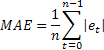
Figure 1 shows a plot of the sum of squares of one-step-ahead forecast errors versus alpha coefficient value for a fragment of test sequence USDJPY M1.

Figure 1. Simple exponential smoothing
The minimum on the resulting plot is barely discernible and is located close to the alpha value of approximately 0.8. But such picture is not always the case with regard to the simple exponential smoothing. When trying to obtain the optimal alpha value for test sequence fragments used in the article, we will more often than not get a plot continuously falling to unity.
Such high values of the smoothing coefficient suggest that this simple model is not quite adequate for the description of our test sequences (quotes). It is either that the process level L(t) changes too fast or there is a trend present in the process.
Let us complicate our model a little by adding another component
![]() ,
,
where:
- X(t) - (simulated) process under study;
- L(t) - variable process level;
- T(t) - linear trend;
- r(t) - zero mean random variable.
It is known that linear regression coefficients can be determined by double smoothening of a sequence:
![]()
![]()
![]()
![]()
For coefficients a1 and a2 obtained in this manner, the m-step-ahead forecast at the time t will be equal to
![]()
It should be noted that the same alpha coefficient is used in the above formulas for the first and repeated smoothing. This model is called the additive one-parameter model of linear growth.
Let us demonstrate the difference between the simple model and the model of linear growth.
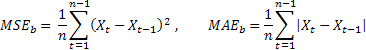
Suppose that for a long time the process under study represented a constant component, i.e. it appeared on the chart as a straight horizontal line but at some point a linear trend started to emerge. A forecast for this process made using the above mentioned models is shown in Figure 2.

Figure 2. Model comparison
As can be seen, the simple exponential smoothing model is appreciably behind the linearly varying input sequence and the forecast made using this model is moving yet further away. We can see a very a different pattern when the linear growth model is used. When the trend emerges, this model is as if trying to come up with the linearly varying sequence and its forecast is closer to the direction of varying input values.
If the smoothing coefficient in the given example was higher, the linear growth model would be able to "reach" the input signal over the given time and its forecast would nearly coincide with the input sequence.
Despite the fact that the linear growth model in the steady state gives good results in the presence of a linear trend, it is easy to see that it takes a certain time for it to "catch up" with the trend. Therefore there will always be a gap between the model and input sequence if the direction of a trend frequently changes. Besides, if the trend grows nonlinearly but instead follows the square law, the linear growth model will not be able to "reach" it. But despite these drawbacks, this model is more beneficial than the simple exponential smoothing model in the presence of a linear trend.
As already mentioned, we used a one-parameter model of linear growth. In order to find the optimal value of the alpha parameter for a fragment of test sequence USDJPY M1, let us build a plot of the sum of squares of one-step-ahead forecast errors versus alpha coefficient value.
This plot built on the basis of the same sequence fragment as the one in Figure 1, is displayed in Figure 3.

Figure 3. Linear growth model
As compared with the result in Figure 1, the optimal value of the alpha coefficient has in this case decreased to approximately 0.4. The first and second smoothing have the same coefficients in this model, although theoretically their values can be different. The linear growth model with two different smoothing coefficients will be reviewed further.
Both exponential smoothing models we considered have their analogs in MetaTrader 5 where they exist in the form of indicators . These are well-known EMA and DEMA which are not designed for forecasting but for smoothing of sequence values.
It should be noted that when using DEMA indicator, a value corresponding to the a1 coefficient is displayed instead of the one-step forecast value. The a2 coefficient (see the above formulas for the linear growth model) is in this case not calculated nor used. In addition, the smoothing coefficient is calculated in terms of the equivalent period n
![]()
For example, alpha equal to 0.8 will correspond to n being approximately equal to 2 and if alpha is 0.4, n is equal to 4.
4. Initial Values
As already mentioned, a smoothing coefficient value shall in one way or another be obtained upon application of exponential smoothing. But this appears to be insufficient. Since in exponential smoothing the current value is calculated on the basis of the previous one, there is a situation where such value does not yet exist at the time zero. In other words, initial value of S or S1 and S2 in the linear growth model shall in some way be calculated at the time zero.
The problem of obtaining initial values is not always easy to solve. If (as in the case of using quotes in MetaTrader 5) we have a very long history available, the exponential smoothing curve will, had the initial values been inaccurately determined, have time to stabilize by a current point, having corrected our initial error. This will require about 10 to 200 (and sometimes even more) periods depending on the smoothing coefficient value.
In this case it would be enough to roughly estimate the initial values and start the exponential smoothing process 200-300 periods before the target time period. It gets more difficult, though, when the available sample only contains e.g. 100 values.
There are various recommendations in literature regarding the choice of initial values. For example, the initial value in the simple exponential smoothing can be equated to the first element in a sequence or calculated as the mean of three to four initial elements in a sequence with a view to smoothing random outliers. The initial values S1 and S2 in the linear growth model can be determined based on the assumption that the initial level of the forecasting curve shall be equal to the first element in a sequence and the slope of the linear trend shall be zero.
One can find yet more recommendations in different sources regarding the choice of initial values but none of them can ensure the absence of noticeable errors at early stages of the smoothing algorithm. It is particularly noticeable with the use of low value smoothing coefficients when a great number of periods is required in order to attain a steady state.
Therefore in order to minimize the impact of problems associated with the choice of initial values (especially for short sequences), we sometimes use a method which involves a search for such values that will result in the minimum forecast error. It is a matter of calculating a forecast error for the initial values varying at small increments over the entire sequence.
The most appropriate variant can be selected after calculating the error within the range of all possible combinations of initial values. This method is however very laborious requiring a lot of calculations and is almost never used in its direct form.
The problem described has to do with optimization or search for a minimum multi-variable function value. Such problems can be solved using various algorithms developed to considerably reduce the scope of calculations required. We will get back to the issues of optimization of smoothing parameters and initial values in forecasting a bit later.
5. Forecast Accuracy Assessment
Forecasting procedure and selection of the model initial values or parameters give rise to the problem of estimating the forecast accuracy. Assessment of accuracy is also important when comparing two different models or determining the consistency of the obtained forecast. There is a great number of well-known estimates for the forecast accuracy assessment but the calculation of any of them requires the knowledge of the forecast error at every step.
As already mentioned, a one-step-ahead forecast error at the time t is equal to
![]()
where:
 – input sequence value at the time t;
 – forecast at the time t made at the previous step.
Probably the most common forecast accuracy estimate is the mean squared error (MSE):

where n is the number of elements in a sequence.
Extreme sensitivity to occasional single errors of large value is sometimes pointed out as a disadvantage of MSE. It derives from the fact that the error value when calculating MSE is squared. As an alternative, it is advisable to use in this case the mean absolute error (MAE).
The squared error here is replaced by the absolute value of the error. It is assumed that the estimates obtained using MAE are more stable.
Both estimates are quite appropriate for e.g. assessment of forecast accuracy of the same sequence using different model parameters or different models but they appear to be of little use for comparison of the forecast results received in different sequences.
Besides, the values of these estimates do not expressly suggest the quality of the forecast result. For example, we cannot say whether the obtained MAE of 0,03 or any other value is good or bad.
To be able to compare the forecast accuracy of different sequences, we can use relative estimates RelMSE and RelMAE:
![]()
The obtained estimates of forecast accuracy are here divided by the respective estimates obtained using the test method of forecasting. As a test method, it is suitable to use the so-called naive method suggesting that the future value of the process will be equal to the current value.
If the mean of forecast errors equals the value of errors obtained using the naive method, the relative estimate value will be equal to one. If the relative estimate value is less than one, it means that, on the average, the forecast error value is less than in the naive method. In other words, the accuracy of forecast results ranks over the accuracy of the naive method. And vice versa, if the relative estimate value is more than one, the accuracy of the forecast results is, on the average, poorer than in the naive method of forecasting.
These estimates are also suitable for assessment of the forecast accuracy for two or more steps ahead. A one-step forecast error in calculations just needs to be replaced with the value of forecast errors for the appropriate number of steps ahead.
As an example, the below table contains one-step ahead forecast errors estimated using RelMAE in one-parameter model of linear growth. The errors were calculated using the last 200 values of each test sequence.
|
Table 1. One-step-ahead forecast errors estimated using RelMAE
RelMAE estimate allows to compare the effectiveness of a selected method when forecasting different sequences. As the results in Table 1 suggest, our forecast was never more accurate than the naive method - all RelMAE values are more than one.
6. Additive Models
There was a model earlier in the article that comprised the sum of the process level, linear trend and a random variable. We will expand the list of the models reviewed in this article by adding another model which in addition to the above components includes a cyclic, seasonal component.
Exponential smoothing models comprising all components as a sum are called the additive models. Apart from these models there are multiplicative models where one, more or all components are comprised as a product. Let us proceed to reviewing the group of additive models.
The one-step-ahead forecast error has repeatedly been mentioned earlier in the article. This error has to be calculated in nearly any application related to forecasting based on exponential smoothing. Knowing the value of the forecast error, the formulas for the exponential smoothing models introduced above can be presented in a somewhat different form (error-correcting form).
The form of the model representation we are going to use in our case contains an error in its expressions that is partially or fully added to the previously obtained values. Such representation is called the additive error model. Exponential smoothing models can also be expressed in a multiplicative error form which will however not be used in this article.
Let us have a look at additive exponential smoothing models.
Simple exponential smoothing:
![]()
![]()
Equivalent model – ARIMA(0,1,1):![]()
Additive linear growth model:
![]()
![]()
![]()
In contrast to the earlier introduced one-parameter linear growth model, two different smoothing parameters are used here.
Equivalent model – ARIMA(0,2,2): ![]()
Linear growth model with damping:
![]()
![]()
![]()
The meaning of such damping is that the trend slope will recede at every subsequent forecasting step depending on the value of the damping coefficient. This effect is demonstrated in Figure 4.

Figure 4. Damping coefficient effect
As can be seen in the figure, when making a forecast, a decreasing value of the damping coefficient will cause the trend to be losing its strength faster, thus the linear growth will get more and more damped.
Equivalent model - ARIMA(1,1,2): ![]()
By adding a seasonal component as a sum to each of these three models we will get three more models.
Simple model with additive seasonality:
![]()
![]()
![]()
Linear growth model with additive seasonality:
![]()
![]()
![]()
![]()
Linear growth model with damping and additive seasonality:
![]()
![]()
![]()
![]()
There are also ARIMA models equivalent to the models with seasonality but they will be left out here as they will hardly have any practical importance whatsoever.
Notations used in the formulas provided are as follows:
 – smoothing parameter for the level of the sequence, [0:1];
 – smoothing parameter for the trend, [0:1];
 – smoothing parameter for seasonal indices, [0:1];
 – damping parameter, [0:1];
 – smoothed level of the sequence calculated at the time t after
  has been observed;
 – smoothed additive trend calculated at the time t;
 – smoothed seasonal index calculated at the time t;
 – value of the sequence at the time t;
- m – number of steps ahead for which the forecast is made;
- p – number of periods in the seasonal cycle;
 – m-step-ahead forecast made at the time t;
 – one-step-ahead forecast error at the time t,
 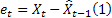 .
.
It is easy to see that the formulas for the last model provided include all six variants under consideration.
If in the formulas for the linear growth model with damping and additive seasonality we take
![]() ,
,
the seasonality will be disregarded in forecasting. Further, where ![]() , a linear growth model will be produced and where
, a linear growth model will be produced and where ![]() , we will get a linear growth model with damping.
, we will get a linear growth model with damping.
The simple exponential smoothing model will correspond to ![]() .
.
When employing the models that involve seasonality, the presence of cyclicity and period of the cycle should first be determined using any available method in order to further use this data for initialization of values of seasonal indices.
We didn't manage to detect a considerable stable cyclicity in the fragments of test sequences used in our case where the forecast is made over short time intervals. Therefore in this article we will not give relevant examples and expand on the characteristics associated with seasonality.
In order to determine the probability prediction intervals with regard to the models under consideration, we will use analytical derivations found in the literature [3]. The mean of the sum of squares of one-step-ahead forecast errors calculated over the entire sample of size n will be used as the estimated variance of such errors.

Then the following expression will be true for determination of the estimated variance in a forecast for 2 and more steps ahead for the models under consideration:
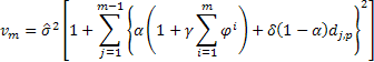
where ![]() equals to one if j modulo p is zero, otherwise
equals to one if j modulo p is zero, otherwise ![]() is zero.
is zero.
Having calculated the estimated variance of the forecast for every step m, we can find the limits of the 95% prediction interval:
![]()
We will agree to name such prediction interval the forecast confidence interval.
Let us implement the expressions provided for the exponential smoothing models in a class written in MQL5.
7. Implementation of the AdditiveES Class
The implementation of the class involved the use of the expressions for the linear growth model with damping and additive seasonality.
As mentioned earlier, other models can be derived from it by an appropriate selection of parameters.
//-----------------------------------------------------------------------------------
//                                                                     AdditiveES.mqh
//                                                                      2011, victorg
//                                                                https://www.mql5.com
//-----------------------------------------------------------------------------------
#property copyright "2011, victorg"
#property link      "https://www.mql5.com"

#include <Object.mqh>

//-----------------------------------------------------------------------------------
// Forecasting. Exponential smoothing. Additive models.
// References:
// 1. Everette S. Gardner Jr. Exponential smoothing: The state of the art – Part II.
//    June 3, 2005.
// 2. Rob J Hyndman. Forecasting based on state space models for exponential
//    smoothing. 29 August 2002.
// 3. Rob J Hyndman et al. Prediction intervals for exponential smoothing
//    using two new classes of state space models. 30 January 2003.
//-----------------------------------------------------------------------------------
class AdditiveES:public CObject
  {
protected:
  double Alpha;    // Smoothed parameter for the level of the series
  double Gamma;    // Smoothed parameter for the trend
  double Phi;      // Autoregressive or damping parameter
  double Delta;    // Smoothed parameter for seasonal indices
  int    nSes;     // Number of periods in the seasonal cycle
  double S;        // Smoothed level of the series, computed after last Y is observed
  double T;        // Smoothed additive trend
  double Ises[];   // Smoothed seasonal indices
  int    p_Ises;   // Pointer for Ises[] shift register
  double F;        // Forecast for 1 period ahead from origin t

public:
         AdditiveES();
  double Init(double s,double t,double alpha=1,double gamma=0,
              double phi=1,double delta=0,int nses=1);
  double GetS()                 { return(S); }
  double GetT()                 { return(T); }
  double GetF()                 { return(F); }
  double GetIs(int m);
  void   IniIs(int m,double is);  // Initialization of smoothed seasonal indices
  double NewY(double y);          // Next calculating step
  double Fcast(int m);            // m-step ahead forecast
  double VarCoefficient(int m);   // Coefficient for calculating prediction intervals

  };
//-----------------------------------------------------------------------------------
// Constructor
//-----------------------------------------------------------------------------------
void AdditiveES::AdditiveES()
  {
  Alpha=0.5; Gamma=0; Delta=0; Phi=1; nSes=1;
  ArrayResize(Ises,nSes);
  ArrayInitialize(Ises,0);
  p_Ises=0; S=0; T=0;
  }
//-----------------------------------------------------------------------------------
// Initialization
//-----------------------------------------------------------------------------------
double AdditiveES::Init(double s,double t,double alpha=1,double gamma=0,
                       double phi=1,double delta=0,int nses=1)
  {
  S=s; T=t;
  Alpha=alpha; if(Alpha<0)Alpha=0; if(Alpha>1)Alpha=1;
  Gamma=gamma; if(Gamma<0)Gamma=0; if(Gamma>1)Gamma=1;
  Phi=phi; if(Phi<0)Phi=0; if(Phi>1)Phi=1;
  Delta=delta; if(Delta<0)Delta=0; if(Delta>1)Delta=1;
  nSes=nses; if(nSes<1)nSes=1;
  ArrayResize(Ises,nSes);
  ArrayInitialize(Ises,0);
  p_Ises=0;
  F=S+Phi*T;
  return(F);
  }
//-----------------------------------------------------------------------------------
// Calculations for the new Y
//-----------------------------------------------------------------------------------
double AdditiveES::NewY(double y)
  {
  double e;

  e=y-F;
  S=S+Phi*T+Alpha*e;
  T=Phi*T+Alpha*Gamma*e;
  Ises[p_Ises]=Ises[p_Ises]+Delta*(1-Alpha)*e;
  p_Ises++; if(p_Ises>=nSes)p_Ises=0;
  F=S+Phi*T+GetIs(0);
  return(F);
  }
//-----------------------------------------------------------------------------------
// Return smoothed seasonal index
//-----------------------------------------------------------------------------------
double AdditiveES::GetIs(int m)
  {
  if(m<0)m=0;
  int i=(int)MathMod(m+p_Ises,nSes);
  return(Ises[i]);
  }
//-----------------------------------------------------------------------------------
// Initialization of smoothed seasonal indices
//-----------------------------------------------------------------------------------
void AdditiveES::IniIs(int m,double is)
  {
  if(m<0)m=0;
  if(m<nSes)
    {
    int i=(int)MathMod(m+p_Ises,nSes);
    Ises[i]=is;
    }
  }
//-----------------------------------------------------------------------------------
// m-step-ahead forecast
//-----------------------------------------------------------------------------------
double AdditiveES::Fcast(int m)
  {
  int i,h;
  double v,v1;

  if(m<1)h=1; else h=m;
  v1=1; v=0;
  for(i=0;i<h;i++){v1=v1*Phi; v+=v1;}
  return(S+v*T+GetIs(h));
  }
//-----------------------------------------------------------------------------------
// Coefficient for calculating prediction intervals
//-----------------------------------------------------------------------------------
double AdditiveES::VarCoefficient(int m)
  {
  int i,h;
  double v,v1,a,sum,k;

  if(m<1)h=1; else h=m;
  if(h==1)return(1);
  v=0; v1=1; sum=0;
  for(i=1;i<h;i++)
    {
    v1=v1*Phi; v+=v1;
    if((int)MathMod(i,nSes)==0)k=1; else k=0;
    a=Alpha*(1+v*Gamma)+k*Delta*(1-Alpha);
    sum+=a*a;
    }
  return(1+sum);
  }
//-----------------------------------------------------------------------------------
Let us briefly review methods of AdditiveES class.
Init method
Input parameters:
- double s - sets the initial value of the smoothed level;
- double t - sets the initial value of the smoothed trend;
- double alpha=1 - sets the smoothing parameter for the level of the sequence;
- double gamma=0 - sets the smoothing parameter for the trend;
- double phi=1 - sets the damping parameter;
- double delta=0 - sets the smoothing parameter for seasonal indices;
- int nses=1 - sets the number of periods in the seasonal cycle.
Returned value:
- It returns a one-step-ahead forecast calculated on the basis of the initial values set.
The Init method shall be called in the first place. This is required for setting the smoothing parameters and initial values. It should be noted that the Init method does not provide for initialization of seasonal indices at arbitrary values; when calling this method, seasonal indices will always be set to zero.
IniIs method
Input parameters:
- Int m - seasonal index number;
- double is - sets the value of the seasonal index number m.
Returned value:
- None
The IniIs(...) method is called when the initial values of seasonal indices need to be other than zero. Seasonal indices should be initialized right after calling the Init(...) method.
NewY method
Input parameters:
- double y – new value of the input sequence
Returned value:
- It returns a one-step-ahead forecast calculated on the basis of the new value of the sequence
This method is designed for calculating a one-step-ahead forecast every time a new value of the input sequence is entered. It should only be called after the class initialization by the Init and, where necessary, IniIs methods.
Fcast method
Input parameters:
- int m – forecasting horizon of 1,2,3,… period;
Returned value:
- It returns the m-step-ahead forecast value.
This method calculates only the forecast value without affecting the state of the smoothing process. It is usually called after calling the NewY method.
VarCoefficient method
Input parameters:
- int m – forecasting horizon of 1,2,3,… period;
Returned value:
- It returns the coefficient value for calculating the forecast variance.
This coefficient value shows the increase in the variance of a m-step-ahead forecast compared to the variance of the one-step-ahead forecast.
GetS, GetT, GetF, GetIs methods
These methods provide access to the protected variables of the class. GetS, GetT and GetF return values of the smoothed level, smoothed trend and a one-step-ahead forecast, respectively. GetIs method provides access to seasonal indices and requires the indication of the index number m as an input argument.
The most complex model out of all we have reviewed is the linear growth model with damping and additive seasonality based on which the AdditiveES class is created. This brings up a very reasonable question - what would the remaining, simpler models be needed.
Despite the fact, that more complex models should seemingly have a clear advantage over simpler ones, it is actually not always the case. Simpler models that have less parameters will in the vast majority of cases result in lesser variance of forecast errors, i.e. their operation will be more steady. This fact is employed in creating forecasting algorithms based on simultaneous parallel operation of all available models, from the simplest to the most complex ones.
Once the sequence have been fully processed, a forecasting model that demonstrated the lowest error, given the number of its parameters (i.e. its complexity), is selected. There is a number of criteria developed for this purpose, e.g. Akaike’s Information Criterion (AIC). It will result in selection of a model which is expected to produce the most stable forecast.
To demonstrate the use of the AdditiveES class, a simple indicator was created all smoothing parameters of which are set manually.
The source code of the indicator AdditiveES_Test.mq5 is set forth below.
//-----------------------------------------------------------------------------------
//                                                                AdditiveES_Test.mq5
//                                                                      2011, victorg
//                                                                https://www.mql5.com
//-----------------------------------------------------------------------------------
#property copyright "2011, victorg"
#property link      "https://www.mql5.com"

#property indicator_chart_window
#property indicator_buffers 4
#property indicator_plots   4

#property indicator_label1  "History"
#property indicator_type1   DRAW_LINE
#property indicator_color1  clrDodgerBlue
#property indicator_style1  STYLE_SOLID
#property indicator_width1  1
#property indicator_label2  "Forecast"      // Forecast
#property indicator_type2   DRAW_LINE
#property indicator_color2  clrDarkOrange
#property indicator_style2  STYLE_SOLID
#property indicator_width2  1
#property indicator_label3  "PInterval+"    // Prediction interval
#property indicator_type3   DRAW_LINE
#property indicator_color3  clrCadetBlue
#property indicator_style3  STYLE_SOLID
#property indicator_width3  1
#property indicator_label4  "PInterval-"    // Prediction interval
#property indicator_type4   DRAW_LINE
#property indicator_color4  clrCadetBlue
#property indicator_style4  STYLE_SOLID
#property indicator_width4  1

double HIST[];
double FORE[];
double PINT1[];
double PINT2[];

input double Alpha=0.2;     // Smoothed parameter for the level
input double Gamma=0.2;     // Smoothed parameter for the trend
input double Phi=0.8;       // Damping parameter
input double Delta=0;       // Smoothed parameter for seasonal indices
input int    nSes=1;        // Number of periods in the seasonal cycle
input int    nHist=250;     // History bars, nHist>=100
input int    nTest=150;     // Test interval, 50<=nTest<nHist
input int    nFore=12;      // Forecasting horizon, nFore>=2

#include "AdditiveES.mqh"
AdditiveES fc;

int    NHist;               // history bars
int    NFore;               // forecasting horizon
int    NTest;               // test interval
double ALPH;                // alpha
double GAMM;                // gamma
double PHI;                 // phi
double DELT;                // delta
int    nSES;                // Number of periods in the seasonal cycle
//-----------------------------------------------------------------------------------
// Custom indicator initialization function
//-----------------------------------------------------------------------------------
int OnInit()
  {
  NHist=nHist; if(NHist<100)NHist=100;
  NFore=nFore; if(NFore<2)NFore=2;
  NTest=nTest; if(NTest>NHist)NTest=NHist; if(NTest<50)NTest=50;
  ALPH=Alpha; if(ALPH<0)ALPH=0; if(ALPH>1)ALPH=1;
  GAMM=Gamma; if(GAMM<0)GAMM=0; if(GAMM>1)GAMM=1;
  PHI=Phi; if(PHI<0)PHI=0; if(PHI>1)PHI=1;
  DELT=Delta; if(DELT<0)DELT=0; if(DELT>1)DELT=1;
  nSES=nSes; if(nSES<1)nSES=1;

  MqlRates rates[];
  CopyRates(NULL,0,0,NHist,rates);           // Load missing data

  SetIndexBuffer(0,HIST,INDICATOR_DATA);
  PlotIndexSetString(0,PLOT_LABEL,"History");
  SetIndexBuffer(1,FORE,INDICATOR_DATA);
  PlotIndexSetString(1,PLOT_LABEL,"Forecast");
  PlotIndexSetInteger(1,PLOT_SHIFT,NFore);
  SetIndexBuffer(2,PINT1,INDICATOR_DATA);
  PlotIndexSetString(2,PLOT_LABEL,"Conf+");
  PlotIndexSetInteger(2,PLOT_SHIFT,NFore);
  SetIndexBuffer(3,PINT2,INDICATOR_DATA);
  PlotIndexSetString(3,PLOT_LABEL,"Conf-");
  PlotIndexSetInteger(3,PLOT_SHIFT,NFore);

  IndicatorSetInteger(INDICATOR_DIGITS,_Digits);
  return(0);
  }
//-----------------------------------------------------------------------------------
// Custom indicator iteration function
//-----------------------------------------------------------------------------------
int OnCalculate(const int rates_total,
                const int prev_calculated,
                const datetime &time[],
                const double &open[],
                const double &high[],
                const double &low[],
                const double &close[],
                const long &tick_volume[],
                const long &volume[],
                const int &spread[])
  {
  int i,j,init,start;
  double v1,v2;

  if(rates_total<NHist){Print("Error: Not enough bars for calculation!"); return(0);}
  if(prev_calculated>rates_total||prev_calculated<=0||(rates_total-prev_calculated)>1)
    {init=1; start=rates_total-NHist;}
  else
    {init=0; start=prev_calculated;}
  if(start==rates_total)return(rates_total);    // New tick but not new bar
//-----------------------
  if(init==1)                                   // Initialization
    {
    i=start;
    v2=(open[i+2]-open[i])/2;
    v1=(open[i]+open[i+1]+open[i+2])/3.0-v2;
    fc.Init(v1,v2,ALPH,GAMM,PHI,DELT,nSES);
    ArrayInitialize(HIST,EMPTY_VALUE);
    }
  PlotIndexSetInteger(1,PLOT_DRAW_BEGIN,rates_total-NFore);
  PlotIndexSetInteger(2,PLOT_DRAW_BEGIN,rates_total-NFore);
  PlotIndexSetInteger(3,PLOT_DRAW_BEGIN,rates_total-NFore);

  for(i=start;i<rates_total;i++)                // History
    {
    HIST[i]=fc.NewY(open[i]);
    }
  v1=0;
  for(i=0;i<NTest;i++)                          // Variance
    {
    j=rates_total-NTest+i;
    v2=close[j]-HIST[j-1];
    v1+=v2*v2;
    }
  v1/=NTest;                                    // v1=var
  j=1;
  for(i=rates_total-NFore;i<rates_total;i++)
    {
    v2=1.96*MathSqrt(v1*fc.VarCoefficient(j));  // Prediction intervals
    FORE[i]=fc.Fcast(j++);                    // Forecasting
    PINT1[i]=FORE[i]+v2;
    PINT2[i]=FORE[i]-v2;
    }

  return(rates_total);
  }
//-----------------------------------------------------------------------------------
A call or a repeated initialization of the indicator sets the exponential smoothing initial values
![]()
There are no initial settings for seasonal indices in this indicator, their initial values are therefore always equal to zero. Upon such initialization, the influence of seasonality on the forecast result will gradually increase from zero to a certain steady value, with the introduction of new incoming values.
The number of cycles required to reach a steady-state operating condition depends on the value of the smoothing coefficient for seasonal indices: the smaller the smoothing coefficient value, the more time it will require.
The operation result of the AdditiveES_Test.mq5 indicator with default settings is shown in Figure 5.

Figure 5. The AdditiveES_Test.mq5 indicator
Apart from the forecast, the indicator displays an additional line corresponding to the one-step forecast for the past values of the sequence and limits of the 95% forecast confidence interval.
The confidence interval is based on the estimated variance of the one-step-ahead error. To reduce the effect of inaccuracy of the selected initial values, the estimated variance is not calculated over the entire length nHist but only with regard to the last bars the number of which is specified in the input parameter nTest.
Files.zip archive at the end of the article includes AdditiveES.mqh and AdditiveES_Test.mq5 files. When compiling the indicator, it is necessary that the include AdditiveES.mqh file is located in the same directory as AdditiveES_Test.mq5.
While the problem of selecting the initial values was to some extent solved when creating the AdditiveES_Test.mq5 indicator, the problem of selecting the optimal values of smoothing parameters has remained open.
8. Selection of the Optimal Parameter Values
The simple exponential smoothing model has a single smoothing parameter and its optimal value can be found using the simple enumeration method. After calculating the forecast error values over the entire sequence, the parameter value is changed at a small increment and a full calculation is made again. This procedure is repeated until all possible parameter values have been enumerated. Now we only need to select the parameter value which resulted in the smallest error value.
In order to find an optimal value of the smoothing coefficient in the range of 0.1 to 0.9 at 0.05 increments, the full calculation of the forecast error value will need to be made seventeen times. As can be seen, the number of calculations required is not so big. But the linear growth model with damping involves the optimization of three smoothing parameters and in this case it will take 4913 calculation runs in order to enumerate all their combinations in the same range at the same 0.05 increments.
The number of full runs required for enumeration of all possible parameter values rapidly increases with the increase in the number of parameters, decrease in the increment and expansion of the enumeration range. Should it further be necessary to optimize the initial values of the models in addition to the smoothing parameters, it will be quite difficult to do using the simple enumeration method.
Problems associated with finding the minimum of a function of several variables are well studied and there is quite a lot of algorithms of this kind. Description and comparison of various methods for finding the minimum of a function can be found in the literature [7]. All these methods are primarily aimed at reducing the number of calls of the objective function, i.e. reducing the computational efforts in the process of finding the minimum.
Different sources often contain a reference to the so-called quasi-Newton methods of optimization. Most likely this has to do with their high efficiency but the implementation of a simpler method should also be sufficient to demonstrate an approach to the optimization of forecasting. Let us opt for Powell's method. Powell's method does not require calculation of derivatives of the objective function and belongs to search methods.
This method, like any other method, may be programmatically implemented in various ways. The search should be completed when a certain accuracy of the objective function value or the argument value is attained. Besides, a certain implementation may include the possibility of using limitations on the permissible range of function parameter changes.
In our case, the algorithm for finding an unconstrained minimum using Powell's method is implemented in PowellsMethod.class. The algorithm stops searching once a given accuracy of the objective function value is attained. In the implementation of this method, an algorithm found in the literature [8] was used as a prototype.
Below is the source code of the PowellsMethod class.
//-----------------------------------------------------------------------------------
//                                                                  PowellsMethod.mqh
//                                                                      2011, victorg
//                                                                https://www.mql5.com
//-----------------------------------------------------------------------------------
#property copyright "2011, victorg"
#property link      "https://www.mql5.com"

#include <Object.mqh>

#define GOLD   1.618034
#define CGOLD  0.3819660
#define GLIMIT 100.0
#define SHFT(a,b,c,d) (a)=(b);(b)=(c);(c)=(d);
#define SIGN(a,b) ((b) >= 0.0 ? fabs(a) : -fabs(a))
#define FMAX(a,b) (a>b?a:b)
//-----------------------------------------------------------------------------------
// Minimization of Functions.
// Unconstrained Powell’s Method.
// References:
// 1. Numerical Recipes in C. The Art of Scientific Computing.
//-----------------------------------------------------------------------------------
class PowellsMethod:public CObject
  {
protected:
  double P[],Xi[];
  double Pcom[],Xicom[],Xt[];
  double Pt[],Ptt[],Xit[];
  int    N;
  double Fret;
  int    Iter;
  int    ItMaxPowell;
  double FtolPowell;
  int    ItMaxBrent;
  double FtolBrent;
  int    MaxIterFlag;
public:
  void   PowellsMethod(void);
  void   SetItMaxPowell(int n)           { ItMaxPowell=n; }
  void   SetFtolPowell(double er)        { FtolPowell=er; }
  void   SetItMaxBrent(int n)            { ItMaxBrent=n;  }
  void   SetFtolBrent(double er)         { FtolBrent=er;  }
  int    Optimize(double &p[],int n=0);
  double GetFret(void)                   { return(Fret);  }
  int    GetIter(void)                   { return(Iter);  }
private:
  void   powell(void);
  void   linmin(void);
  void   mnbrak(double &ax,double &bx,double &cx,double &fa,double &fb,double &fc);
  double brent(double ax,double bx,double cx,double &xmin);
  double f1dim(double x);
  virtual double func(const double &p[]) { return(0); }
  };
//-----------------------------------------------------------------------------------
// Constructor
//-----------------------------------------------------------------------------------
void PowellsMethod::PowellsMethod(void)
  {
  ItMaxPowell= 200;
  FtolPowell = 1e-6;
  ItMaxBrent = 200;
  FtolBrent  = 1e-4;
  }
//-----------------------------------------------------------------------------------
void PowellsMethod::powell(void)
  {
  int i,j,m,n,ibig;
  double del,fp,fptt,t;

  n=N; Fret=func(P);
  for(j=0;j<n;j++)Pt[j]=P[j];
  for(Iter=1;;Iter++)
    {
    fp=Fret; ibig=0; del=0.0;
    for(i=0;i<n;i++)
      {
      for(j=0;j<n;j++)Xit[j]=Xi[j+n*i];
      fptt=Fret;
      linmin();
      if(fabs(fptt-Fret)>del){del=fabs(fptt-Fret); ibig=i;}
      }
    if(2.0*fabs(fp-Fret)<=FtolPowell*(fabs(fp)+fabs(Fret)+1e-25))return;
    if(Iter>=ItMaxPowell)
      {
      Print("powell exceeding maximum iterations!");
      MaxIterFlag=1; return;
      }
    for(j=0;j<n;j++){Ptt[j]=2.0*P[j]-Pt[j]; Xit[j]=P[j]-Pt[j]; Pt[j]=P[j];}
    fptt=func(Ptt);
    if(fptt<fp)
      {
      t=2.0*(fp-2.0*(Fret)+fptt)*(fp-Fret-del)*(fp-Fret-del)-del*(fp-fptt)*(fp-fptt);
      if(t<0.0)
        {
        linmin();
        for(j=0;j<n;j++){m=j+n*(n-1); Xi[j+n*ibig]=Xi[m]; Xi[m]=Xit[j];}
        }
      }
    }
  }
//-----------------------------------------------------------------------------------
void PowellsMethod::linmin(void)
  {
  int j,n;
  double xx,xmin,fx,fb,fa,bx,ax;

  n=N;
  for(j=0;j<n;j++){Pcom[j]=P[j]; Xicom[j]=Xit[j];}
  ax=0.0; xx=1.0;
  mnbrak(ax,xx,bx,fa,fx,fb);
  Fret=brent(ax,xx,bx,xmin);
  for(j=0;j<n;j++){Xit[j]*=xmin; P[j]+=Xit[j];}
  }
//-----------------------------------------------------------------------------------
void PowellsMethod::mnbrak(double &ax,double &bx,double &cx,
                                 double &fa,double &fb,double &fc)
  {
  double ulim,u,r,q,fu,dum;

  fa=f1dim(ax); fb=f1dim(bx);
  if(fb>fa)
    {
    SHFT(dum,ax,bx,dum)
    SHFT(dum,fb,fa,dum)
    }
  cx=bx+GOLD*(bx-ax); fc=f1dim(cx);
  while(fb>fc)
    {
    r=(bx-ax)*(fb-fc); q=(bx-cx)*(fb-fa);
    u=bx-((bx-cx)*q-(bx-ax)*r)/(2.0*SIGN(FMAX(fabs(q-r),1e-20),q-r));
    ulim=bx+GLIMIT*(cx-bx);
    if((bx-u)*(u-cx)>0.0)
      {
      fu=f1dim(u);
      if(fu<fc){ax=bx; bx=u; fa=fb; fb=fu; return;}
      else if(fu>fb){cx=u; fc=fu; return;}
      u=cx+GOLD*(cx-bx); fu=f1dim(u);
      }
    else if((cx-u)*(u-ulim)>0.0)
      {
      fu=f1dim(u);
      if(fu<fc)
        {
        SHFT(bx,cx,u,cx+GOLD*(cx-bx))
        SHFT(fb,fc,fu,f1dim(u))
        }
      }
    else if((u-ulim)*(ulim-cx)>=0.0){u=ulim; fu=f1dim(u);}
      else {u=cx+GOLD*(cx-bx); fu=f1dim(u);}
    SHFT(ax,bx,cx,u)
    SHFT(fa,fb,fc,fu)
    }
  }
//-----------------------------------------------------------------------------------
double PowellsMethod::brent(double ax,double bx,double cx,double &xmin)
  {
  int    iter;
  double a,b,d,e,etemp,fu,fv,fw,fx,p,q,r,tol1,tol2,u,v,w,x,xm;

  a=(ax<cx?ax:cx); b=(ax>cx?ax:cx);
  d=0.0; e=0.0; x=w=v=bx; fw=fv=fx=f1dim(x);
  for(iter=1;iter<=ItMaxBrent;iter++)
    {
    xm=0.5*(a+b); tol2=2.0*(tol1=FtolBrent*fabs(x)+2e-19);
    if(fabs(x-xm)<=(tol2-0.5*(b-a))){xmin=x; return(fx);}
    if(fabs(e)>tol1)
      {
      r=(x-w)*(fx-fv); q=(x-v)*(fx-fw);
      p=(x-v)*q-(x-w)*r; q=2.0*(q-r);
      if(q>0.0)p=-p; q=fabs(q);
      etemp=e; e=d;
      if(fabs(p)>=fabs(0.5*q*etemp)||p<=q*(a-x)||p>=q*(b-x))
        d=CGOLD*(e=(x>=xm?a-x:b-x));
      else {d=p/q; u=x+d; if(u-a<tol2||b-u<tol2)d=SIGN(tol1,xm-x);}
      }
    else d=CGOLD*(e=(x>=xm?a-x:b-x));
    u=(fabs(d)>=tol1?x+d:x+SIGN(tol1,d));
    fu=f1dim(u);
    if(fu<=fx)
      {
      if(u>=x)a=x; else b=x;
      SHFT(v,w,x,u)
      SHFT(fv,fw,fx,fu)
      }
    else
      {
      if(u<x)a=u; else b=u;
      if(fu<=fw||w==x){v=w; w=u; fv=fw; fw=fu;}
      else if(fu<=fv||v==x||v==w){v=u; fv=fu;}
      }
    }
  Print("Too many iterations in brent");
  MaxIterFlag=1; xmin=x;
  return(fx);
  }
//-----------------------------------------------------------------------------------
double PowellsMethod::f1dim(double x)
  {
  int j;
  double f;

  for(j=0;j<N;j++) Xt[j]=Pcom[j]+x*Xicom[j];
  f=func(Xt);
  return(f);
  }
//-----------------------------------------------------------------------------------
int PowellsMethod::Optimize(double &p[],int n=0)
  {
  int i,j,k,ret;

  k=ArraySize(p);
  if(n==0)N=k;
  else N=n;
  if(N<1||N>k)return(0);
  ArrayResize(P,N); ArrayResize(Xi,N*N);
  ArrayResize(Pcom,N); ArrayResize(Xicom,N);
  ArrayResize(Xt,N); ArrayResize(Pt,N);
  ArrayResize(Ptt,N); ArrayResize(Xit,N);
  for(i=0;i<N;i++)for(j=0;j<N;j++)Xi[i+N*j]=(i==j?1.0:0.0);
  for(i=0;i<N;i++)P[i]=p[i];
  MaxIterFlag=0;
  powell();
  for(i=0;i<N;i++)p[i]=P[i];
  if(MaxIterFlag==1)ret=-1;
  else ret=Iter;
  return(ret);
  }
//-----------------------------------------------------------------------------------
The Optimize method is the main method of the class.
Optimize method
Input parameters :
- double &p[] - array that at the input contains the initial values of parameters the optimal values of which shall be found; the obtained optimal values of these parameters are at the output of the array.
- int n=0 - number of arguments in array p[]. Where n=0, the number of parameters is considered to be equal to the size of array p[].
Returned value:
- It returns the number of iterations required for operation of the algorithm, or -1 if the maximum permissible number thereof has been reached.
When searching for optimal parameter values, an iterative approximation to the minimum of the objective function occurs. The Optimize method returns the number of iterations required to reach the function minimum with a given accuracy. The objective function is called several times at every iteration, i.e. the number of calls of the objective function may be significantly (ten and even hundred times) bigger than the number of iterations returned by the Optimize method.
Other methods of the class.
SetItMaxPowell method
Input parameters:
- Int n - maximum permissible number of iterations in Powell's method. The default value is 200.
Returned value:
- None.
It sets the maximum permissible number of iterations; once this number is reached, the search will be over regardless of whether the minimum of the objective function with a given accuracy was found. And a relevant message will be added to the log.
SetFtolPowell method
Input parameters:
- double er - accuracy. Should this value of deviation from the minimum value of the objective function be reached, Powell's method stops searching. The default value is 1e-6.
Returned value:
- None.
SetItMaxBrent method
Input parameters:
- Int n - maximum permissible number of iterations for an auxiliary Brent's method. The default value is 200.
Returned value:
- None.
It sets the maximum permissible number of iterations. Once it is reached, the auxiliary Brent's method will stop searching and a relevant message will be added to the log.
SetFtolBrent method
Input parameters:
- double er – accuracy. This value defines accuracy in the search of the minimum for the auxiliary Brent's method. The default value is 1e-4.
Returned value:
- None.
GetFret method
Input parameters:
- None.
Returned value:
- It returns the minimum value of the objective function obtained.
GetIter method
Input parameters:
- None.
Returned value:
- It returns the number of iterations required for operation of the algorithm.
Virtual function func(const double &p[])
Input parameters:
- const double &p[] – address of the array containing the optimized parameters. The size of the array corresponds to the number of function parameters.
Returned value:
- It returns the function value corresponding to the parameters passed to it.
The virtual function func() shall in every particular case be redefined in a class derived from the PowellsMethod class. The func() function is the objective function the arguments of which corresponding to the minimum value returned by the function will be found when applying the search algorithm.
This implementation of Powell's method employs Brent's univariate parabolic interpolation method for determining the direction of search with regard to each parameter. The accuracy and maximum permissible number of iterations for these methods can be set separately by calling SetItMaxPowell, SetFtolPowell, SetItMaxBrent and SetFtolBrent.
So the default characteristics of the algorithm can be changed in this manner. This may appear useful when the default accuracy set to a certain objective function turns out to be too high and the algorithm requires too many iterations in the search process. The change in the value of the required accuracy can optimize the search with regard to different categories of objective functions.
Despite the seeming complexity of the algorithm that employs Powell's method, it is quite simple in use.
Let us review an example. Assume, we have a function
![]()
and we need to find the values of parameters ![]() and
and ![]() at which the function will have the smallest value.
at which the function will have the smallest value.
Let us write a script demonstrating a solution to this problem.
//-----------------------------------------------------------------------------------
//                                                                        PM_Test.mq5
//                                                                      2011, victorg
//                                                                https://www.mql5.com
//-----------------------------------------------------------------------------------
#property copyright "2011, victorg"
#property link      "https://www.mql5.com"

#include "PowellsMethod.mqh"
//-----------------------------------------------------------------------------------
class PM_Test:public PowellsMethod
  {
public:
  void   PM_Test(void) {}
private:
  virtual double func(const double &p[]);
  };
//-----------------------------------------------------------------------------------
double PM_Test::func(const double &p[])
  {
  double f,r1,r2;

  r1=p[0]-0.5;
  r2=p[1]-6.0;
  f=r1*r1*4.0+r2*r2;
  return(f);
  }
//-----------------------------------------------------------------------------------
// Script program start function
//-----------------------------------------------------------------------------------
void OnStart()
  {
  int it;
  double p[2];

  p[0]=8; p[1]=9;                                 // Initial point
  PM_Test *pm = new PM_Test;
  it=pm.Optimize(p);
  Print("Iter= ",it,"        Fret= ",pm.GetFret());
  Print("p[0]= ",p[0],"    p[1]= ",p[1]);
  delete pm;
  }
//-----------------------------------------------------------------------------------
When writing this script, we first create the func() function as a member of the PM_Test class which calculates the value of the given test function using the passed values of parameters p[0] and p[1]. Then in the body of the OnStart() function, the initial values are assigned to the required parameters. The search will start from these values.
Further, a copy of the PM_Test class is created and the search for the required values of p[0] and p[1] starts by calling the Optimize method; the methods of the parent PowellsMethod class will call the redefined func() function. Upon completion of the search, the number of iterations, function value at the minimum point and the obtained parameter values p[0]=0.5 and p[1]=6 will be added to the log.
PowellsMethod.mqh and a test case PM_Test.mq5 are located at the end of the article in Files.zip archive. In order to compile PM_Test.mq5, it should be located in the same directory as PowellsMethod.mqh.
9. Optimization of the Model Parameter Values
The previous section of the article dealt with implementation of the method for finding the function minimum and gave a simple example of its use. We will now proceed to the issues related to optimization of the exponential smoothing model parameters.
For a start, let us simplify the earlier introduced AdditiveES class to the maximum by excluding from it all elements associated with the seasonal component, as the models that take into consideration seasonality are not going to be further considered in this article anyway. This will allow to make the source code of the class much easier to comprehend and reduce the number of calculations. In addition, we will also exclude all calculations related to forecasting and computations of the forecast confidence intervals for an easy demonstration of an approach to the optimization of parameters of the linear growth model with damping under consideration.
//-----------------------------------------------------------------------------------
//                                                                     OptimizeES.mqh
//                                                                      2011, victorg
//                                                                https://www.mql5.com
//-----------------------------------------------------------------------------------
#property copyright "2011, victorg"
#property link      "https://www.mql5.com"

#include "PowellsMethod.mqh"
//-----------------------------------------------------------------------------------
// Class OptimizeES
//-----------------------------------------------------------------------------------
class OptimizeES:public PowellsMethod
  {
protected:
  double Dat[];            // Input data
  int    Dlen;             // Data lenght
  double Par[5];           // Parameters
  int    NCalc;            // Number of last elements for calculation
public:
  void   OptimizeES(void) {}
  int    Calc(string fname);
private:
  int    readCSV(string fnam,double &dat[]);
  virtual double func(const double &p[]);
  };
//-----------------------------------------------------------------------------------
// Calc
//-----------------------------------------------------------------------------------
int OptimizeES::Calc(string fname)
  {
  int i,it;
  double relmae,naiv,s,t,alp,gam,phi,e,ae,pt;

  if(readCSV(fname,Dat)<0){Print("Error."); return(-1);}
  Dlen=ArraySize(Dat);
  NCalc=200;                               // number of last elements for calculation
  if(NCalc<0||NCalc>Dlen-1){Print("Error."); return(-1);}
  Par[0]=Dat[Dlen-NCalc];                  // initial S
  Par[1]=0;                                // initial T
  Par[2]=0.5;                              // initial Alpha
  Par[3]=0.5;                              // initial Gamma
  Par[4]=0.5;                              // initial Phi
  it=Optimize(Par);                        // Powell's optimization
  s=Par[0]; t=Par[1]; alp=Par[2]; gam=Par[3]; phi=Par[4];
  relmae=0; naiv=0;
  for(i=Dlen-NCalc;i<Dlen;i++)
    {
    e=Dat[i]-(s+phi*t);
    relmae+=MathAbs(e); naiv+=MathAbs(Dat[i]-Dat[i-1]);
    ae=alp*e; pt=phi*t; s=s+pt+ae; t=pt+gam*ae;
    }
  relmae/=naiv;
  PrintFormat("%s:    N=%i,  RelMAE=%.3f",fname,NCalc,relmae);
  PrintFormat("Iter= %i,  Fmin= %e",it,GetFret());
  PrintFormat("p[0]= %.5f,  p[1]= %.5f,  p[2]= %.2f,  p[3]= %.2f,  p[4]= %.2f",
                                             Par[0],Par[1],Par[2],Par[3],Par[4]);
  return(0);
  }
//-----------------------------------------------------------------------------------
// readCSV
//-----------------------------------------------------------------------------------
int OptimizeES::readCSV(string fnam,double &dat[])
  {
  int n,asize,fhand;

  fhand=FileOpen(fnam,FILE_READ|FILE_CSV|FILE_ANSI);
  if(fhand==INVALID_HANDLE)
    {
    Print("FileOpen Error!");
    return(-1);
    }
  asize=512;
  ArrayResize(dat,asize);
  n=0;
  while(FileIsEnding(fhand)!=true)
    {
    dat[n++]=FileReadNumber(fhand);
    if(n+128>asize)
      {
      asize+=128;
      ArrayResize(dat,asize);
      }
    }
  FileClose(fhand);
  ArrayResize(dat,n-1);
  return(0);

  }
//------------------------------------------------------------------------------------
// func
//------------------------------------------------------------------------------------
double OptimizeES::func(const double &p[])
  {
  int i;
  double s,t,alp,gam,phi,k1,k2,k3,e,sse,ae,pt;

  s=p[0]; t=p[1]; alp=p[2]; gam=p[3]; phi=p[4]; k1=1; k2=1; k3=1;
  if     (alp>0.95){k1+=(alp-0.95)*200; alp=0.95;}                 // Alpha   > 0.95
  else if(alp<0.05){k1+=(0.05-alp)*200; alp=0.05;}                 // Alpha   < 0.05
  if     (gam>0.95){k2+=(gam-0.95)*200; gam=0.95;}                 // Gamma   > 0.95
  else if(gam<0.05){k2+=(0.05-gam)*200; gam=0.05;}                 // Gamma   < 0.05
  if     (phi>1.0 ){k3+=(phi-1.0 )*200; phi=1.0; }                 // Phi     > 1.0
  else if(phi<0.05){k3+=(0.05-phi)*200; phi=0.05;}                 // Phi     < 0.05
  sse=0;
  for(i=Dlen-NCalc;i<Dlen;i++)
    {
    e=Dat[i]-(s+phi*t); sse+=e*e;
    ae=alp*e; pt=phi*t; s=s+pt+ae; t=pt+gam*ae;
    }
  return(NCalc*MathLog(k1*k2*k3*sse));
  }
//------------------------------------------------------------------------------------
The OptimizeES class derives from the PowellsMethod class and includes redefining of the virtual function func(). As mentioned earlier, the parameters whose calculated value will be minimized in the course of optimization shall be passed at the input of this function.
In accordance with the maximum likelihood method, the func() function calculates the logarithm of the sum of squares of one-step-ahead forecast errors. The errors are calculated in a loop with regard to NCalc recent values of the sequence.
To preserve the stability of the model, we should impose limitations on the range of changes in its parameters. This range for Alpha and Gamma parameters will be from 0.05 to 0.95, and for Phi parameter - from 0.05 to 1.0. But for optimization in our case, we use a method for finding an unconstrained minimum which does not imply the use of limitations on the arguments of the objective function.
We will try to turn the problem of finding the minimum of the multi-variable function with limitations into a problem of finding an unconstrained minimum, to be able to take into consideration all limitations imposed on the parameters without changing the search algorithm. For this purpose, the so-called penalty function method will be used. This method can easily be demonstrated for a one-dimensional case.
Suppose that we have a function of a single argument (whose domain is from 2.0 to 3.0) and an algorithm which in the search process can assign any values to this function parameter. In this case, we can do as follows: if the search algorithm has passed an argument which exceeds the maximum permissible value, e.g. 3.5, the function can be calculated for the argument equal to 3.0 and the obtained result is further multiplied by a coefficient proportional to the excess of the maximum value, for example k=1+(3.5-3)*200.
If similar operations are performed with regard to argument values that turned out to be below the minimum permissible value, the resulting objective function is guaranteed to increase outside the permissible range of changes in its argument. Such artificial increase in the resulting value of the objective function allows to keep the search algorithm unaware of the fact that the argument passed to the function was in any way limited and guarantee that the minimum of the resulting function will be within the set limits of the argument. Such approach is easily applied to a function of several variables.
The main method of the OptimizeES class is the Calc method. A call of this method is responsible for reading data from a file, search for optimal parameter values of a model and estimation of the forecast accuracy using RelMAE for the obtained parameter values. The number of processed values of the sequence read from a file is in this case set in the variable NCalc.
Below is the example of the Optimization_Test.mq5 script that uses the OptimizeES class.
//-----------------------------------------------------------------------------------
//                                                              Optimization_Test.mq5
//                                                                      2011, victorg
//                                                                https://www.mql5.com
//-----------------------------------------------------------------------------------
#property copyright "2011, victorg"
#property link      "https://www.mql5.com"

#include "OptimizeES.mqh"

OptimizeES es;
//-----------------------------------------------------------------------------------
// Script program start function
//-----------------------------------------------------------------------------------
void OnStart()
  {
  es.Calc("Dataset\\USDJPY_M1_1100.TXT");
  }
//-----------------------------------------------------------------------------------
Following the execution of this script, the obtained result will be as shown below.

Figure 6. Optimization_Test.mq5 script result
Although we can now find optimal parameter values and initial values of the model, there is yet one parameter which cannot be optimized using simple tools - the number of sequence values used in optimization. In optimization with regard to a sequence of great length, we will obtain the optimal parameter values that, on the average, ensure a minimum error over the entire length of the sequence.
However if the nature of the sequence varied within this interval, the obtained values for some of its fragments will no longer be optimal. On the other hand, if the sequence length is dramatically decreased, there is no guarantee that the optimal parameters obtained for such a short interval will be optimal over a longer time lag.
OptimizeES.mqh and Optimization_Test.mq5 are located at the end of the article in Files.zip archive. When compiling, it is necessary that OptimizeES.mqh and PowellsMethod.mqh are located in the same directory as the compiled Optimization_Test.mq5. In the given example, USDJPY_M1_1100.TXT file is used that contains the test sequence and that should be located in the directory \MQL5\Files\Dataset\.
Table 2 shows the estimates of the forecast accuracy obtained using RelMAE by means of this script. Forecasting was done with regard to eight test sequences mentioned earlier in the article using the last 100, 200 and 400 values of each of these sequences.
|
Table 2. Forecast errors estimated using RelMAE
As can be seen, the forecast error estimates are close to unity but in the majority of cases the forecast for the given sequences in this model is more accurate than in the naive method.
10. The IndicatorES.mq5 Indicator
The AdditiveES_Test.mq5 indicator based on the AdditiveES.mqh class was mentioned earlier upon review of the class. All smoothing parameters in this indicator were set manually.
Now after considering the method allowing to optimize the model parameters, we can create a similar indicator where the optimal parameter values and initial values will be determined automatically and only the processed sample length will need to be set manually. That said, we will exclude all calculations related to seasonality.
The source code of the CIndiсatorES class used in creating the indicator is set forth below.
//-----------------------------------------------------------------------------------
//                                                                   CIndicatorES.mqh
//                                                                      2011, victorg
//                                                                https://www.mql5.com
//-----------------------------------------------------------------------------------
#property copyright "2011, victorg"
#property link      "https://www.mql5.com"

#include "PowellsMethod.mqh"
//-----------------------------------------------------------------------------------
// Class CIndicatorES
//-----------------------------------------------------------------------------------
class CIndicatorES:public PowellsMethod
  {
protected:
  double Dat[];                                              // Input data
  int    Dlen;                                               // Data lenght
  double Par[5];                                             // Parameters
public:
  void   CIndicatorES(void)       { }
  void   CalcPar(double &dat[]);
  double GetPar(int n)            { if(n>=0||n<5)return(Par[n]); else return(0); }
private:
  virtual double func(const double &p[]);
  };
//-----------------------------------------------------------------------------------
// CalcPar
//-----------------------------------------------------------------------------------
void CIndicatorES::CalcPar(double &dat[])
  {

  Dlen=ArraySize(dat);
  ArrayResize(Dat,Dlen);
  ArrayCopy(Dat,dat);

  Par[0]=Dat[0];                                             // initial S
  Par[1]=0;                                                  // initial T
  Par[2]=0.5;                                                // initial Alpha
  Par[3]=0.5;                                                // initial Gamma
  Par[4]=0.5;                                                // initial Phi
  Optimize(Par);                                             // Powell's optimization
  }
//------------------------------------------------------------------------------------
// func
//------------------------------------------------------------------------------------
double CIndicatorES::func(const double &p[])
  {
  int i;
  double s,t,alp,gam,phi,k1,k2,k3,e,sse,ae,pt;

  s=p[0]; t=p[1]; alp=p[2]; gam=p[3]; phi=p[4]; k1=1; k2=1; k3=1;
  if     (alp>0.95){k1+=(alp-0.95)*200; alp=0.95;}           // Alpha   > 0.95
  else if(alp<0.05){k1+=(0.05-alp)*200; alp=0.05;}           // Alpha   < 0.05
  if     (gam>0.95){k2+=(gam-0.95)*200; gam=0.95;}           // Gamma   > 0.95
  else if(gam<0.05){k2+=(0.05-gam)*200; gam=0.05;}           // Gamma   < 0.05
  if     (phi>1.0 ){k3+=(phi-1.0 )*200; phi=1.0; }           // Phi     > 1.0
  else if(phi<0.05){k3+=(0.05-phi)*200; phi=0.05;}           // Phi     < 0.05
  sse=0;
  for(i=0;i<Dlen;i++)
    {
    e=Dat[i]-(s+phi*t); sse+=e*e;
    ae=alp*e; pt=phi*t; s=s+pt+ae; t=pt+gam*ae;
    }
  return(Dlen*MathLog(k1*k2*k3*sse));
  }
//------------------------------------------------------------------------------------
This class contains CalcPar and GetPar methods; the first one is designed for calculation of the optimal parameter values of the model, the second one is intended for accessing those values. Besides, the CIndicatorES class comprises the redefining of the virtual function func().
The source code of the IndicatorES.mq5 indicator:
//-----------------------------------------------------------------------------------
//                                                                    IndicatorES.mq5
//                                                                      2011, victorg
//                                                                https://www.mql5.com
//-----------------------------------------------------------------------------------
#property copyright "2011, victorg"
#property link      "https://www.mql5.com"

#property indicator_chart_window
#property indicator_buffers 4
#property indicator_plots   4

#property indicator_label1  "History"
#property indicator_type1   DRAW_LINE
#property indicator_color1  clrDodgerBlue
#property indicator_style1  STYLE_SOLID
#property indicator_width1  1
#property indicator_label2  "Forecast"                 // Forecast
#property indicator_type2   DRAW_LINE
#property indicator_color2  clrDarkOrange
#property indicator_style2  STYLE_SOLID
#property indicator_width2  1
#property indicator_label3  "ConfUp"                   // Confidence interval
#property indicator_type3   DRAW_LINE
#property indicator_color3  clrCrimson
#property indicator_style3  STYLE_DOT
#property indicator_width3  1
#property indicator_label4  "ConfDn"                   // Confidence interval
#property indicator_type4   DRAW_LINE
#property indicator_color4  clrCrimson
#property indicator_style4  STYLE_DOT
#property indicator_width4  1

input int nHist=80; // History bars, nHist>=24

#include  "CIndicatorES.mqh"
#define   NFORE 12

double    Hist[],Fore[],Conf1[],Conf2[];
double    Data[];
int       NDat;

CIndicatorES   Es;
//-----------------------------------------------------------------------------------
// Custom indicator initialization function
//-----------------------------------------------------------------------------------
int OnInit()
  {
  NDat=nHist; if(NDat<24)NDat=24;
  MqlRates rates[];
  CopyRates(NULL,0,0,NDat,rates);                   // Load missing data
  ArrayResize(Data,NDat);

  SetIndexBuffer(0,Hist,INDICATOR_DATA);
  PlotIndexSetString(0,PLOT_LABEL,"History");
  SetIndexBuffer(1,Fore,INDICATOR_DATA);
  PlotIndexSetString(1,PLOT_LABEL,"Forecast");
  PlotIndexSetInteger(1,PLOT_SHIFT,NFORE);
  SetIndexBuffer(2,Conf1,INDICATOR_DATA);            // Confidence interval
  PlotIndexSetString(2,PLOT_LABEL,"ConfUp");
  PlotIndexSetInteger(2,PLOT_SHIFT,NFORE);
  SetIndexBuffer(3,Conf2,INDICATOR_DATA);            // Confidence interval
  PlotIndexSetString(3,PLOT_LABEL,"ConfDN");
  PlotIndexSetInteger(3,PLOT_SHIFT,NFORE);
  IndicatorSetInteger(INDICATOR_DIGITS,_Digits);
  return(0);
  }
//-----------------------------------------------------------------------------------
// Custom indicator iteration function
//-----------------------------------------------------------------------------------
int OnCalculate(const int rates_total,
                const int prev_calculated,
                const datetime &time[],
                const double &open[],
                const double &high[],
                const double &low[],
                const double &close[],
                const long &tick_volume[],
                const long &volume[],
                const int  &spread[])
  {
  int i,start;
  double s,t,alp,gam,phi,e,f,a,a1,a2,a3,var,ci;

  if(rates_total<NDat){Print("Error: Not enough bars for calculation!"); return(0);}
  if(prev_calculated==rates_total)return(rates_total); // New tick but not new bar
  start=rates_total-NDat;
//-----------------------
  PlotIndexSetInteger(0,PLOT_DRAW_BEGIN,rates_total-NDat);
  PlotIndexSetInteger(1,PLOT_DRAW_BEGIN,rates_total-NFORE);
  PlotIndexSetInteger(2,PLOT_DRAW_BEGIN,rates_total-NFORE);
  PlotIndexSetInteger(3,PLOT_DRAW_BEGIN,rates_total-NFORE);

  for(i=0;i<NDat;i++)Data[i]=open[rates_total-NDat+i]; // Input data
  Es.CalcPar(Data);                                    // Optimization of parameters
  s=Es.GetPar(0); t=Es.GetPar(1); alp=Es.GetPar(2); gam=Es.GetPar(3); phi=Es.GetPar(4);
  f=(s+phi*t); var=0;
  for(i=0;i<NDat;i++)                                // History
    {
    e=Data[i]-f; var+=e*e;
    a1=alp*e; a2=phi*t; s=s+a2+a1; t=a2+gam*a1;
    f=(s+phi*t); Hist[start+i]=f;
    }
  var/=(NDat-1); a1=1; a2=0; a3=1;
  for(i=rates_total-NFORE;i<rates_total;i++)
    {
    a1=a1*phi; a2+=a1;
    Fore[i]=s+a2*t;                                 // Forecast
    ci=1.96*MathSqrt(var*a3);                        // Confidence intervals
    a=alp*(1+a2*gam); a3+=a*a;
    Conf1[i]=Fore[i]+ci;
    Conf2[i]=Fore[i]-ci;
    }
  return(rates_total);
  }
//-----------------------------------------------------------------------------------
With every new bar, the indicator finds the optimal values of the model parameters, makes calculations in the model for a given number of bars NHist, builds a forecast and defines the forecast confidence limits.
The only parameter of the indicator is the length of the processed sequence the minimum value of which is limited to 24 bars. All calculations in the indicator are made on the basis of the open[] values. The forecasting horizon is 12 bars. The code of the IndicatorES.mq5 indicator and CIndicatorES.mqh file are located at the end of the article in Files.zip archive.

Figure 7. Operation result of the IndicatorES.mq5 indicator
An example of the operation result of the IndicatorES.mq5 indicator is shown in Figure 7. In the course of operation of the indicator, the 95% forecast confidence interval will take values corresponding to the obtained optimal parameter values of the model. The bigger the smoothing parameter values, the faster the increase in the confidence interval upon the increasing forecasting horizon.
With a simple improvement, the IndicatorES.mq5 indicator can be used not only for forecasting currency quotes but also for forecasting values of various indicators or preprocessed data.
Conclusion
The main objective of the article was to familiarize the reader with additive exponential smoothing models used in forecasting. While demonstrating their practical use, some accompanying issues were also dealt with. However the materials provided in the article can be considered merely an introduction to the large range of problems and solutions associated with forecasting.
I would like to draw your attention to the fact that the classes, functions, scripts and indicators provided were created in the process of writing the article and are primarily designed to serve as examples to the materials of the article. Therefore no serious testing for stability and errors was performed. Besides, the indicators set forth in the article should be considered to be only a demonstration of the implementation of the methods involved.
The forecast accuracy of the IndicatorES.mq5 indicator introduced in the article can most likely be somewhat improved by using the modifications of the applied model which would be more adequate in terms of peculiarities of the quotes under consideration. The indicator can also be amplified by other models. But these issues fall beyond the scope of this article.
In conclusion, it should be noted that exponential smoothing models can in certain cases produce forecasts of the same accuracy as the forecasts obtained by applying more complex models thus proving once again that even the most complex model is not always the best.
References
- Everette S. Gardner Jr. Exponential Smoothing: The State of the Art – Part II. June 3, 2005.
- Rob J Hyndman. Forecasting Based on State Space Models for Exponential Smoothing. 29 August 2002.
- Rob J Hyndman et al. Prediction Intervals for Exponential Smoothing Using Two New Classes of State Space Models. 30 January 2003.
- Rob J Hyndman and Muhammad Akram. Some Nonlinear Exponential Smoothing Models Are Unstable. 17 January 2006.
- Rob J Hyndman and Anne B Koehler. Another Look at Measures of Forecast Accuracy. 2 November 2005.
- Yu. P. Lukashin. Adaptive Methods for Short-Term Forecasting of Time Series: Textbook. - М.: Finansy i Statistika, 2003.-416 pp.
- D. Himmelblau. Applied Nonlinear Programming. М.: Mir, 1975.
- Numerical Recipes in C. The Art of Scientific Computing. Second Edition. Cambridge University Press.
Translated from Russian by MetaQuotes Ltd.
Original article: https://www.mql5.com/ru/articles/318
Warning: All rights to these materials are reserved by MetaQuotes Ltd. Copying or reprinting of these materials in whole or in part is prohibited.
This article was written by a user of the site and reflects their personal views. MetaQuotes Ltd is not responsible for the accuracy of the information presented, nor for any consequences resulting from the use of the solutions, strategies or recommendations described.

 Create Your Own Graphical Panels in MQL5
 Speed Up Calculations with the MQL5 Cloud Network
 Analysis of the Main Characteristics of Time Series
- Free trading apps
- Over 8,000 signals for copying
- Economic news for exploring financial markets
You agree to website policy and terms of use
I have only finished reading the chapter on additive models. So it is, to put it mildly, too early to summarise. However, some comments arose as I was reading:
Continue reading....
Finished reading it. Great article, thanks! More comments:
Becoming a Fearless Forex Trader
- Must You Know What Will Happen Next?
- Is There a Better Way?
- Strategies When You Know That You Don’t Know
“Good investing is a peculiar balance between the conviction to follow your ideas and the flexibility to recognize when you have made a mistake.”-Michael Steinhardt
"95% of the trading errors you are likely to make will stem from your attitudes about being wrong, losing money, missing out, and leaving money on the table – the four trading fears"
-Mark Douglas, Trading In the Zone
Many traders become enamored with the idea of forecasting. The need for forecasting seems to be inherent to successful trading. After all, you reason, I must know what will happen next in order to make money, right? Thankfully, that’s not right and this article will break down how you can trade well without knowing what will happen next.
Must You Know What Will Happen Next?
While knowing what would happen next would be helpful, no one can know for sure. The reason that insider trading is a crime that is often tested in equity markets can help you see that some traders are so desperate to know the future that their willing to cheat and pay a stiff fine when caught. In short, it’s dangerous to think in terms of a certain future when your money is on the line and best to think of edges over certainties when taking a trade.
The problem with thinking that you must know what the future holds for your trade, is that when something adverse happens to your trade from your expectations, fear sets in. Fear in and of itself isn’t bad. However, most traders with their money on the line, will often freeze and fail to close out the trade.
If you don’t need to know what will happen next, what do you need? The list is surprisingly short and simple but what’s more important is that you don’t think you know what will happen because if you do, you’ll likely overleverage and downplay the risks which are ever-present in the world of trading.
- A Clean Edge That You’re Comfortable Entering A Trade On
- A Well Defined Invalidation Point Where Your Trade Set-Up No Longer
- A Potential Reversal Entry Point
- An Appropriate Trade Size / Money Management
Is There a Better Way?Yesterday, the European Central Bank decided to cut their refi rate and deposit rate. Many traders went into this meeting short, yet EURUSD covered ~250% of its daily ATR range and closed near the highs, indicating EURUSD strength. Simply put, the outcome was outside of most trader’s realm of possibility and if you went short and were struck by fear, you likely did not close out that short and were another “victim of the market”, which is another way of saying a victim of your own fears of losing.
So what is the better way? Believe it or not, it’s to approach the market, understanding how emotional markets can be and that it is best not to get tied up in the direction the market “has to go”. Many traders will hold on to a losing trade, not to the benefit of their account, but rather to protect their ego. Of course, the better path to trading is to focus on protecting your account equity and leaving your ego at the door of your trading room so that it does not affect your trading negatively.
Strategies When You Know That You Don’t Know
There is one commonality with traders who can trade without fear. They build losing trades into their approach. It’s similar to a gambit in chess and it takes away the edge and strong-hold that fear has on many traders. For those non-chess players, a gambit is a play in which you sacrifice a low-value piece, like a pawn, for the sake of gaining an advantage. In trading, the gambit could be your first trade that allows you to get a better taste of the edge you’re sensing at the moment the trade is entered.
James Stanley’s USD Hedge is a great example of a strategy that works under the assumption that one trade will be a loser. What’s the significance of this? It pre-assumes the loss and will allow you to trade without the fear that plagues so many traders. Another tool that you can use to help you define if the trend is staying in your favor or going against you is a fractal.
If you look outside of the world of trading and chess, there are other businesses that presume a loss and therefore are able to act with a clear head when a loss comes. Those businesses are casinos and insurance companies. Both of these businesses presume a loss and work only in line with a calculated risk, they operate free of fear and you can as well if you presume small losses as part of your strategy.
Another great Mark Douglas quote:
“The less I cared about whether or not I was wrong, the clearer things became, making it much easier to move in and out of positions, cutting my losses short to make myself mentally available to take the next opportunity.” -Mark Douglas
Happy Trading!
The source
I agree that one does not need to know what will happen next in order to profit, but the question seems to be in defining an edge. Casinos define their edge using predefined probabilities, e.g., there's a 1/52 chance of drawing an Ace of Spades from a complete standard deck of cards, or a 1/6 chance of rolling a 5 using a fair dice. Insurance companies use aggregate histories to compile actuarial tables from which to make assumptions regarding populations, but cannot (much like traders) make assumptions regarding any particular individual without knowing some facts regarding behavioral habits of the individual to compare to the attributes of the population. 20 year old males tend to be aggressive, somewhat reckless drivers; John is a 20 year old male, he "may" be an aggressive, somewhat reckless driver, but there is also a chance that he may not be. The insurance company will then look at John's driving record for any history of risky behavior, very much like a trader looks at price history to determine exploitable "behaviors."
So as a trader, much more like insurance companies than casinos, we gather information regarding the past to attempt to make assumptions about the future when defining our edge. Combining the entry/exit conditions with risk management to make assertions regarding unknowable probabilities (because one cannot assert that there is a 1/6 chance that the EURUSD will increase by 20 pips with 100% confidence) is the essence of trading. So it all boils down to making the most of the time available to an individual trader, finding the most advantageous setups/exits using assumptions regarding price histories and profit/loss expectancies should the future be similar to the past, which is uncertain at best.
Using an exponentially smoothed time series forecast as a setup/exit together with risk management is no different really than using a consolidation/breakout strategy in that one creates rules for the trade based on how the strategy worked in the past, and then follows the rules with as few assumptions regarding the future as possible.
Will price go up, or will it go down? I don't know, but this is what I'll do in either case.