Introduction to the Empirical Mode Decomposition Method

Introduction

All real processes we have to deal with in practice are complex, as a rule, consisting of a great number of components. For example, weather. When analyzing precipitation charts, we should bear in mind that they represent interaction between a lot of various processes such as seasonal changes, global warming/cooling processes, ocean current changes, dynamics of cyclones and anticyclones, the amount of carbon dioxide emitted into the atmosphere, solar activity cycles, etc. The list could go on forever.

A chart of this type is therefore quite difficult to be analyzed as its components, when interacting with each other, mask and distort the regularities we would like to identify. This gives rise to a rightful desire to break down the process under consideration into individual components and analyze each of the components separately. Analysis of individual components and consideration of the contribution they make into the process at hand helps us better understand the process in progress, as well as, e.g. increase the forecast reliability.

And there is no exception when it comes to various information on trading, including currency quotes that are also formed based on a great number of different factors. That is why it is quite natural to expect that an upfront breakdown into individual components can greatly facilitate their further analysis.

The term "decomposition" formally means the breaking down of a compound process or a composite material into separate constituent components. But in many areas related to analysis of different processes, signal analysis, analysis of various sorts of sequences, etc., this term has long been used in a broader meaning very often suggesting not a breakdown into actual initial components but rather a breakdown into certain functions that were not actually present when the initial data was being formed. These functions are sort of artificially formed in the process of data decomposition but despite their "artificial" origin they allow for a deeper analysis of data helping to identify hidden patterns.

The vast majority of methods used in market analysis can explicitly or implicitly be attributed to methods that single out certain components from the analyzed process, i.e. decomposition methods. Let us briefly review some of them.

1. Decomposition

There is a lot of various decomposition methods that can be applied in practice to a given sequence under consideration. These methods may have different underlying mathematical or empirical approaches, different degree of complexity and different areas of application.

For example, even a fundamental market analysis can - at a certain stretch - be considered one of decomposition methods. This analysis deals with the effect produced by a set of initial events that directly influence market conditions. In other words, an analyzed market process is implicitly decomposed into a number of events that make it up.

Issues related to fundamental analysis will not be touched upon later on. We will assume that any further information on the process under consideration is not available; what we have is only a sequence representing the behavior of a given process

The simplest decomposition example can be illustrated by a decomposition of a sequence into several components using the usual well-known methods. For example, we plot a MA on a chart for any currency pair. Then subtract the resulting curve from the initial sequence. As a result, we will get two components of the initial sequence, the MA curve and the residue. The same procedure, only using a longer period MA, when applied to the obtained residue, will result in three components - two MA curves and the residue of the transform. As you can see, the process of decomposition can easily be arranged using any means available. The whole point lies in properties of the results of such a process.

Among well known decomposition and spectral analysis methods, the Fourier transform is definitely worth mentioning here. The Fourier transform belongs to the class of orthogonal transformations that uses fixed harmonic basis functions. The Fourier transform result can be shown as a decomposition of the initial process into harmonic functions with fixed frequencies and amplitudes. Note two points of particular importance to us.

First, the transform is always performed in a fixed, priorly set basis of orthogonal functions. That is, a transform basis does not depend on the nature of a transformed sequence.

Second, amplitude and frequency values of the resulting harmonic components are constant. That is, their values are constant over the entire initial sequence. This means that if the nature of a given initial sequence was changing over an interval under consideration, such changes will not be reflected in the transform results. The results obtained in this case will only reflect a certain averaged state of the process as this transform is based on the assumption of stationarity of the initial data.

To avoid constraints associated with non-stationarity of the initial sequence, we can switch from the Fourier transform over to a wavelet transform. A wavelet transform, like the Fourier transform, performs decomposition in a fixed basis of functions. Unlike the Fourier transform, this basis shall be preset, i.e. a wavelet used in transform shall be selected.

Further, in contrast to the Fourier transform, every component resulting from a wavelet transform has parameters that determine its scale and level over time which solves the problem associated with a possible non-stationarity of an analyzed process.

The Fourier transform and wavelet transform both have received wide recognition due to well established mathematical techniques used and effective implementation algorithms available. Besides, both transforms appear to be quite versatile and can successfully be applied in different areas.

But for practical purposes, it would be good to have a transform that would not only allow to deal with non-stationary processes but would also use an adaptive transform basis determined by initial data. This type of transform does exist and will be briefly considered below thus addressing the main subject of this article.

2. Empirical Mode Decomposition

The Empirical Mode Decomposition (EMD) was proposed as the fundamental part of the Hilbert–Huang transform (HHT). The Hilbert Huang transform is carried out, so to speak, in 2 stages. First, using the EMD algorithm, we obtain intrinsic mode functions (IMF).

Then, at the second stage, the instantaneous frequency spectrum of the initial sequence is obtained by applying the Hilbert transform to the results of the above step. The HHT allows to obtain the instantaneous frequency spectrum of nonlinear and nonstationary sequences. These sequences can consequently also be dealt with using the empirical mode decomposition.

However, this article is not going to cover the plotting of the instantaneous frequency spectrum using the Hilbert transform. We will focus only on the EMD algorithm.

In contrast to the previously mentioned Fourier transform and wavelet transform, the EMD decomposes any given data into intrinsic mode functions (IMF) that are not set analytically and are instead determined by an analyzed sequence alone. The basis functions are in this case derived adaptively directly from input data. An IMF resulting from the EMD shall satisfy only the following requirements:

1. The number of IMF extrema (the sum of the maxima and minima) and the number of zero-crossings must either be equal or differ at most by one;
2. At any point of an IMF the mean value of the envelope defined by the local maxima and the envelope defined by the local minima shall be zero.

Decomposition results in a family of frequency ordered IMF components. Each successive IMF contains lower frequency oscillations than the preceding one. And although the term "frequency" is not quite correct when used in relation to IMFs, it is probably best suited to define their nature. The thing is that even though an IMF is of oscillatory nature, it can have variable amplitude and frequency along the time axis.

It is quite difficult to visualize the EMD algorithm performance results based on the description alone so let us proceed to its software implementation that will give us an opportunity to get to know the algorithm peculiarities.

3. EMD Algorithm

The algorithm as proposed by Huang is based on producing smooth envelopes defined by local maxima and minima of a sequence and subsequent subtraction of the mean of these envelopes from the initial sequence. This requires the identification of all local extrema that are further connected by cubic spline lines to produce the upper and the lower envelopes.

The procedure of plotting the envelopes is shown in Figure 1.

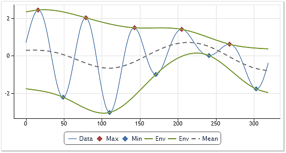
Fig. 1. Plotting the envelopes and their mean

Figure 1 gives the analyzed sequence in the thin blue line. The maxima and minima of the sequence are shown in red and blue, respectively. The envelopes are given in green.

The mean is calculated based on the two envelopes and is shown in Figure 1 as the dashed line. The mean value so calculated is further subtracted from the initial sequence.

The above steps result in the extraction of the required empirical function in the first approximation. To obtain the final IMF, new maxima and minima shall again be identified and all the above steps repeated. This repeated process is called sifting. The sifting process is repeated until a certain given stoppage criterion is met. Selection of sifting stoppage criteria is one of the key points affecting the decomposition result as a whole. We will get back to the discussion of this issue a bit later.

If the sifting process is successfully completed, we will get the first IMF. The next IMF can be obtained by subtracting the previously extracted IMF from the original signal and repeating the above described procedure once again. This continues until all IMFs are extracted. The sifting process usually stops when the residue, for example, contains no more than two extrema.

As can be seen, the described empirical mode decomposition procedure is not based on strict mathematical computations but is rather truly empirical, thus fully justifying its name. Despite the simplicity and clarity of the above algorithm as proposed by Huang, there is a few points that can be regarded as its downsides.

Various publications on this subject provide detailed reviews of its weak points, as well as ways of modernizing the Huang's algorithm. This article is not going to focus on possible modernizations of this method but will simply demonstrate an attempt to create its software implementation. The implementation peculiarities will be briefly outlined below.

4. CEMDecomp Class

The CEMDecomp class implementing the EMD algorithm was created based on the Internet publications devoted to the Hilbert-Huang transform and empirical mode decomposition. The implemented algorithm is substantially very similar to the algorithm initially proposed by Huang and does not contain any major modifications.

Below is a snippet of the source code that can be found in the CEMDecomp.mqh file at the end of the article.

//------------------------------------------------------------------------------------
// The Empirical Mode Decomposition (EMD).
//------------------------------------------------------------------------------------
class CEMDecomp:public CObject
  {
public:
  int     N;                 // Input and output data size
  double  Mean;              // Mean of input data
  int     nIMF;              // IMF counter
  int     MaxIMF;            // Maximum number of IMF
  int     MaxIter;           // Maximum number of iterations
  int     FixedIter;         // 0-variable number of sifting iterations;
                             // 1-always ten sifting iterations.
  double  IMFResult[];       // Result
private:
  double  X[];
  double  Imf[];
  double  XMax[];            // x of local maxima
  double  YMax[];            // y of local maxima
  double  XMin[];            // x of local minima
  double  YMin[];            // y of local minima
  double  EnvUpp[];          // Upper envelope
  double  EnvLow[];          // Lower envelope
  double  Eps;               // Accuracy comparison of floating-point numbers
  double  Tol;               // Accuracy of calculation IMF
public:  
  void    CEMDecomp(void);
  int     Decomp(double &y[]);          // Decomposition
  void    GetIMF(double &x[], int nn);  // Get IMF number nn
private:
  int     arrayprepare(void);
  void    extrema(double &y[],int &nmax,double &xmax[],double &ymax[], int &nmin,double &xmin[],double &ymin[]);
  int     SplineInterp(double &x[],double &y[],int n,double &x2[], double &y2[],int btype=0);
  };

Let us have a look at public variables and methods declared in the CEMDecomp class.

N is the number of elements in the sequence. The value of the variable N is generated after calling the Decomp() method and is equal to the input sequence length. The extracted IMFs will have the same size.

Mean is the mean value of the input sequence. The value is generated after calling the Decomp() method.

nIMF is the IMF counter. After calling Decomp(), it contains the number of extracted IMFs plus two. Thus, this value indicates how many components can be read using the GetIMF() method. That said, a component with 0 index will always contain the initial sequence from which its mean value is subtracted, while a component with index nIMF will contain the residue of decomposition.

MaxIMF is the maximum permissible number of IMFs. Decomposition of the input sequence into separate IMFs will stop, when the number of IMF's reaches the MaxIMF value. The value of this variable can be set before calling the Decomp() method. The default value is 16.

MaxIter is the maximum number of iterations allowed in the sifting process. If the number of iterations in the sifting process reaches this value, the sifting will stop regardless of whether or not the required accuracy has been achieved. The value of this variable can be set before calling the Decomp() method. The default value is 2000.

FixedIter is the flag that sets a stoppage criterion in sifting. If the FixedIter value is zero, the sifting process for each IMF will stop once the given accuracy is achieved. The number of iterations required to achieve the given accuracy for the extraction of different IMFs may vary. If the FixedIter is set to one, an IMF will always be extracted in 10 iterations. The value of this variable can be set before calling the Decomp() method. The default value is 0.

Decomp(double &y[]) is the main class method carrying out the decomposition. It receives a reference to an array containing input data, as an input parameter. Upon successful completion, the variable N will be equal to the input array length. The extracted IMFs will have the same size. The variable Mean will be equal to the mean value of the input sequence, while the variable nIMF will be equal to the number of components that can be read using the GetIMF() method.

GetIMF(double &x[], int nn) serves to ensure access to the results obtained using the Decomp() method. The address of the array where the component with the number set by nn will be copied into is passed as an input parameter. That said, a component with 0 index will always contain the initial sequence from which its mean value is subtracted, while a component with index nIMF will contain the residue of decomposition. If the array length passed as a parameter turns out to be smaller than the length of the resulting components, the array will be filled as much as its length allows.

The use of the CEMDecomp class can be demonstrated by the following example:

#include "CEMDecomp.mqh"
//------------------------------------------------------------------------------------
// Script program start function
//------------------------------------------------------------------------------------
void OnStart()
  {
  int n,ret;
  double yy[],imf2[];
  
  n=400;                                    // Input sequence length
  ArrayResize(yy,n);                         // Array of input data
  ArrayResize(imf2,n);                       // Array for reading the results
  
  CopyOpen(_Symbol,PERIOD_CURRENT,0,n,yy);      // Generation of input data
  
  CEMDecomp *emd=new CEMDecomp();           // Creation of the CEMDecomp class instance
  ret=emd.Decomp(yy);                       // Decomposition of the input sequence
  
  if((ret==0)&&(emd.nIMF>3))                // If there is no error and the sufficient
                                            // number of components was extracted,
    emd.GetIMF(imf2,2);                     // copy component number 2 into
                                            // array imf2[].
  delete(emd);                              // Deletion of the CEMDecomp class instance
  
  // One of the extracted components in array imf2[].
  }
//------------------------------------------------------------------------------------

A full example of decomposition displaying extracted IMFs through Web interface can be found in the CEMDecomposition.zip archive at the end of the article. To run this example, you should unpack the specified archive and place the whole \CEMDecomposition directory together with its contents into the \Indicators or \Scripts directory of the terminal. Afterwards, you can compile and run the EMDecomp_Test.mq5 script. Keep in mind that the use of external libraries in the terminal should in so doing be allowed.

Figure 2 shows another example featuring decomposition of USDJPY Daily quotes with the sequence length of 100 elements. It can be seen, that the decomposition of this sequence resulted in extraction of four IMFs and the residue.

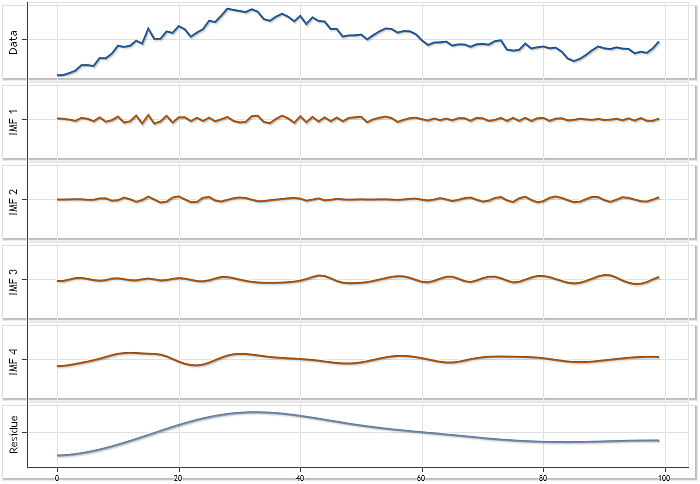
Fig. 2. Decomposition of the sequence of USDJPY Daily quotes, where N=100

All the charts in Figure 2 are displayed in the same scale allowing to evaluate the contribution made by each of the extracted IMFs. However this way of plotting cannot give a sufficiently clear picture to see the peculiarities of each of the IMFs. Figure 3 demonstrates the same results, only using auto scaling mode for each of the charts.

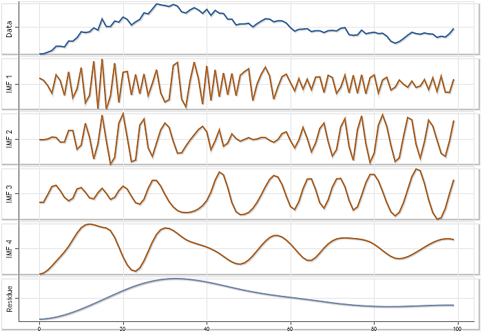
Fig. 3. Decomposition of the sequence of USDJPY Daily quotes, where N=100. Auto scaling mode

And although Figure 3 does not display the actual correlation of amplitudes of the individual components, the use of the auto scaling mode allows for a more detailed visualization of every one of them.

5. Notes to the Proposed Implementation of the EMD Algorithm

The first thing I would like to draw your attention to is the method for identification of maxima and minima of the initial sequence. In this case, there are two options available.

Figure 4 shows performance results of the algorithm for identification of extrema.

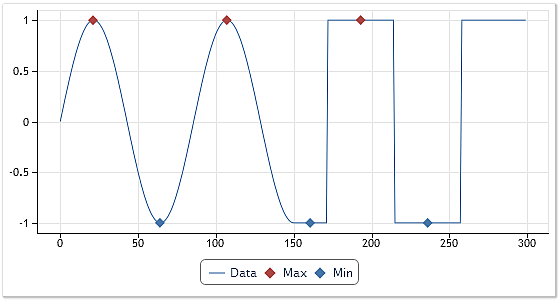
Fig. 4. Identification of extrema. The first option

When it comes to identification of maxima or minima of a function, the algorithm that is most commonly used is as follows:

1. The value of the current element of the sequence is compared with the preceding and subsequent values;
2. If the current value is greater than the preceding and the subsequent value, it is identified as the function maximum;
3. If the current value is smaller than the preceding and the subsequent value, it is identified as the function minimum;

For sequences with clearly defined extrema, the identification of maxima and minima does not involve any difficulty. The algorithm provided works just fine. This case is demonstrated in the first half of the chart shown in Figure 4. However this algorithm will be unresponsive to flat tops where the nearest values of the sequence are equal.

Had the provided algorithm been used, the last maximum and two last minima shown in Figure 4 would have never been identified. On the one hand, this result would have been expected and correct. But on the other, drawing the analogy to oscillatory processes, if zero-crossings occurred, these extrema would have been overlooked. It is not quite clear whether the flat tops of a rectangular sequence or sections of equal sequence values can be considered extrema.

Nevertheless, the algorithm used for identification of extrema when implementing the EMDecomp class is an improved version of the algorithm provided above. Its performance results can be observed in Figure 4. This algorithm identifies intervals with equal sequence values as extrema and places points of extremum in the middle of these intervals.

The algorithm for identification of maxima and minima whose performance results are shown in Figure 4 is used in the CEMDecomp class for calculation of the number of extrema when determining the point where the decomposition cycle should stop. For example, if an IMF extracted does not have any extremum, the decomposition stops and such IMF is cast out.

Should this identification algorithm be used when plotting envelopes, then, in cases where the input sequence, for example, takes the form as shown in Fig. 4, the resulting envelopes will be represented by two straight parallel lines. The sifting process will further fail to transform the input sequence and this input sequence will, in turn, not be suitable for decomposition into components.

A way out of this situation can be found in the use of a somewhat different algorithm for identification of extrema to plot the envelopes.

Figure 5 demonstrates the results obtained using this alternative algorithm for identification of extrema.

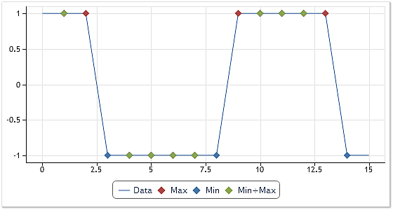
Fig.  5. Identification of extrema. The second option

Let us have a closer look at Figure 5. Unlike Figure 4, it shows green points being maxima and minima at the same time. If envelopes are plotted based on these extrema, they will no longer be straight parallel lines and hidden components of the rectangular sequence will be available for further extraction in the sifting process. A good illustration of the above can be a test case located in the CEMDecomposition.zip archive at the end of the article.

Unfortunately, this approach does not solve all the problems related to extraction of hidden components. For example, hidden components cannot be extracted in this manner for a triangular sequence. This fact can be one of the downsides of this implementation of the EMD algorithm. This difficult situation can probably be tackled by switching to the CEEMD (The Complementary Ensemble Empirical Mode Decomposition Method) algorithm for decomposition the review of which is not covered in this article.

Apart from the peculiarities associated with implementation of algorithms for identifying extrema, attention should also be given to the problem of end effects typical of this kind of algorithms. To elaborate on the above, let us turn to Fig. 1. Figure 1 clearly shows that the maxima are connected by a cubic interpolating spline function as the upper envelope.

That said, the envelope should be defined for the sections located both to the left of the first maximum and to the right of the last maximum. The way in which such envelope is elongated is likely to determine the nature of IMFs extracted next to its ends. Without going into much detail of the software implementation of end effect correction, this fact is simply brought here to the reader's attention.

We should further note that the nature and number of extracted IMFs can and will depend on the method selected to stop the sifting cycle. The CEMDecomp class uses the calculation of the ratio indicating the extent of the difference in the current IMF as determined by the last sifting cycle as the main method that serves to stop the sifting process.

If the sifting has almost no effect on an unknown IMF, the sifting process stops and the IMF is considered to be produced. A limiting value by default determining the IMF extraction accuracy is set in the class constructor. Having set the default limiting value, the number of sifting iterations can sometimes reach 200 and even 300. In publications on this subject, many authors warn against using such a great number of sifting iterations. It was nevertheless decided to use this default limiting value in this implementation of the EMD algorithm.

This implementation of the EMD algorithm allows to use another stoppage criterion. For this purpose, the variable FixedIter should be set to 1 before calling the Decomp() method. In this case, all IMFs will always be extracted in 10 sifting iterations. And it is easy to see that the decomposition results obtained using this stoppage criterion will be somewhat different versus those of the default method .

6. Application of the EMD Algorithm

Since the EMD algorithm was initially a part of the Hilbert-Huang transform, the calculation of the instantaneous frequency spectrum of a sequence can serve as an example demonstrating the application of this algorithm. This involves performance of the Hilbert transform on IMF components extracted using the EMD. This procedure is however not considered in this article.

Apart from calculating the spectrum, the EMD algorithm can be used to smooth sequences.

Figure 6 shows an example of such smoothing.

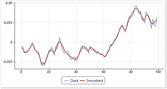
Fig. 6. Smoothing of the input sequence

An arbitrary fragment of USDCHF Daily quotes consisting of 100 "Open" price values was selected for smoothing. In the process of decomposition, four IMFs and the residue were obtained. All IMFs, except for the first one, were further added to the residue.

Thus, the highest-frequency component found was excluded from the input sequence. If we disregarded the first two components when adding them up, the resulting curve would be even smoother.

Another example of the EMD application can be generation of a forecast based on IMFs extracted from the input sequence. To generate a forecast, you can use any extrapolator whereby a forecast is generated for each of IMFs and the residue separately.

The forecasts generated in this manner are then added up to produce the required forecast result for the input sequence. Considering the oscillatory nature of individual IMFs, we can suppose that to generate a forecast, it would be reasonable to use extrapolators taking into account the periodic behavior of forecast sequences.

In our case, we will review an example of operation of a simpler extrapolator where a forecast for each of IMFs will be generated using 10-step-ahead linear extrapolation. The result of this forecast is shown in Figure 7.

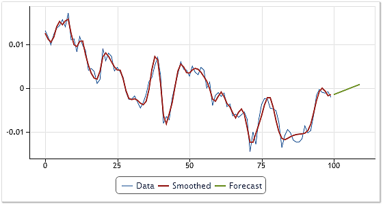
Fig. 7. Generating a forecast for USDCHF, H4 quotes

It should be noted that when generating a forecast, one or more highest-frequency components can be discarded. Thus, the effect of high-frequency noise on the forecast can be mitigated. The result of the forecast that excludes the first IMF is demonstrated in Figure 7. Forecastability of this method was in this case not assessed. A detailed analysis of forecasting methods that are based on the empirical mode decomposition is not provided here as this subject lies beyond the scope of this article.

We cannot but mention detrending, too. After the individual sequence components are obtained using the EMD, a fairly flexible algorithm can be developed for detrending. The residue of decomposition or the residue added to one or more of the last extracted IMFs can be taken as a trend. The number of IMFs involved in creating of a trend line together with the residue may vary depending on the number of low-frequency components required to remain in the sequence after detrending.

Thus, to detrend, it is enough to add up all IMFs extracted as a result of the decomposition, except for the last component or several last components. This procedure can easily be combined with smoothing of the obtained result, if the highest-frequency component is also excluded from the process of adding up the components. Figure 8 shows an example of detrending using the above technique.

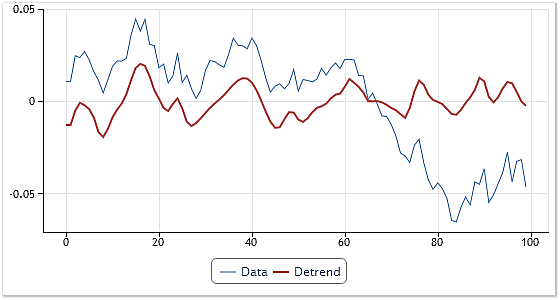
Fig. 8. Detrending combined with smoothing

A sequence of EURUSD, Daily quotes was taken as the initial data. Following the decomposition, all the extracted components were added up, excluding the residue of decomposition, the last and the first IMFs. It resulted not only in detrending but also in a certain smoothing of the resulting curve.

The area of application of the empirical mode decomposition method is certainly not limited to the simple examples given in the article. But since this article focuses more on the issues of implementation of the EMD method as such, rather than its application, let us consider the examples provided herein below.

Figure 9 demonstrating the decomposition result obtained using the parameters set in CEMDecomp.mqh by default can serve as an additional illustration of functionality offered by this implementation of the EMD method. This example is based on the use of XAUUSD H4 quotes. The sequence length is 150 elements.

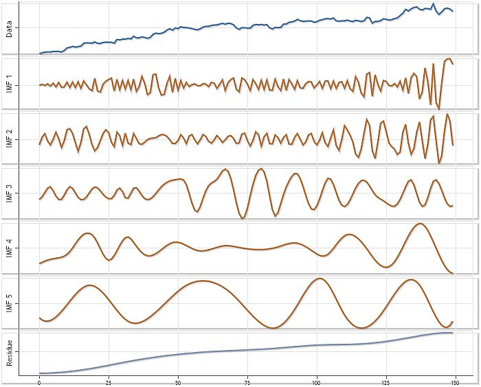
Fig. 9. Decomposition example using XAUUSD H4 quotes

Auto scaling was applied to each of the components in Figure 9.

Conclusion

Remember that the empirical mode decomposition method, as well as the Hilbert–Huang transform, is intended for analyzing data from nonstationary and nonlinear processes. It does not mean that this approach cannot be applied to linear and stationary sequences.

A few approaches used in decomposition algorithms were briefly touched upon at the beginning of the article. And it was mentioned that the majority of these algorithms decompose a sequence into components that do not in fact represent initial processes actually making up the sequence under consideration.

These components are in some way synthetic; their extraction merely helps to better understand the structure of an input sequence and in many cases allows to facilitate its analysis. The EMD method is no exception. You should never think that the components obtained using this method reflect the actual physical processes out of which the initial analyzed data was originally formed.

The implementation proposed in this article may probably require further testing and improvement as it can hardly be considered ideal.

The main objective of this article was however to familiarize the reader with the EMD method and some peculiarities related to its implementation.

Summing things up.

1. The article very briefly touches upon some general decomposition-related issues;
2. In a few words it sets forth the essence of the empirical mode decomposition method;
3. The listing and a short description of the CEMDecomp class interface where the EMD method is implemented are introduced;
4. The example of interaction with the CEMDecomp class also demonstrating how its methods are called is given;
5. Some peculiarities of the proposed implementation of the EMD method are outlined;
6. A few simple examples demonstrating the application of the EMD method in data analysis are provided;
7. At the end of the article, you can find the CEMDecomp.mqh file implementing the EMD method, as well as the EMDecomposition.zip archive containing the full test case featuring the use of the CEMDecomp class.

References

1. Hilbert-Huang transform.
2. Hilbert-Huang transform.
3. Empirical Mode Decomposition.

Annex

The original article was published on June 28, 2012. This annex was offered on July 5, 2012.

An alternative EMD method implementation is offered as an addition to the article. That implementation is displayed as CEMD class and placed in CEMD_2.mqh file attached below.