Self Optimizing Expert Advisor With MQL5 And Python (Part IV): Stacking Models

In this series of articles, we will discuss different ways of building trading applications capable of dynamically adjusting themselves to evolving market conditions. There are potentially infinite ways we can approach this problem but, it is unlikely that all possible solutions will be valid. Therefore, our goal today is to demonstrate and empirically analyze the merits and shortcomings of different possible solutions, to help you improve your trading strategies.

Overview of The Trading Strategy

We shall turn our attention to forecasting the NZDJPY currency pair. We desire to algorithmically learn a trading strategy from the data we will collect on the symbol from our MetaTrader 5 Terminal. As humans, we may be naturally biased towards trading strategies that are aligned with our own beliefs and interests. Machine learning models are also biased. The bias of a machine learning model, is the extent to which the assumptions made by the model are violated. Our trading strategy will rely on an ensemble of 2 AI models. The first model will be trained to predict the future close price of the NZDJPY pair, 20 minutes into the future. The second model will be trained to predict the amount of error in the prediction made by the first model. This technique is known as stacking. Our hope is that by stacking 2 models, we will be able to overcome our human bias, and hopefully this will be enough to lead us to higher levels of performance.

Overview of The Methodology

We fetched approximately, 9000 rows of M1 market data on the NZDJPY pair from our MetaTrader 5 Terminal using a customized MQL5 script. We created 2D and 3D scatter plots of the market data. However, we were not able to identify any discernible relationships in the data. We also performed time-series decomposition on the data-set, and we were able to identify a clear downtrend and the presence of strong seasonal effects in the data.

Our data was then partitioned into training and test sets. A set of 15 different models were fit and evaluated on the training set. The Stochastic Gradient Descent (SGD) Regressor was the bet performing model from the group.

Subsequently, when we analyzed our feature importance metrics, we found that the High price appeared to be the most informative predictor we had for predicting the future close price of the NZDJPY pair. The High price obtained the best Mutual Information (MI) score. Furthermore, we also employed scikit-learn’s implementation of the Recursive Feature Elimination (RFE) algorithm. All the predictors we have were deemed important by the RFE algorithm. However, as we shall see in our discussion, just because a relationship exists, does not guarantee we will successfully capture and model it.

After identifying our best performing model, we then proceeded to tune the parameters of our model. Normally in our discussions, after parameter tuning, we usually proceed to test for overfitting by comparing the performance of our customized model against the performance of the default model. However, there are many different ways we can test for overfitting. Today, we chose to test for overfitting by analyzing our model’s residuals. We observed high levels of correlation between our model’s residuals and its lags. Normally, the residuals of a model that has sufficiently learned should have no correlation. Therefore, this suggested to us that our best performing model may not have learned effectively, or that there exists other data that may help us explain our target, and we have failed to include that data.

Afterward, we recorded the residuals of our model on the training and test sets. We did not fit the model on the test set at this point. We then cross validated our set of 15 models on the training residuals of our SGD Regressor. Our best performing model was the Lasso Regression, however we selected the third-best model, a Deep Neural Network (DNN), as our candidate solution. Our rationale for doing so was the flexibility offered to us by the deep neural network gives us an opportunity to tune it better to the data, than we could tune the Lasso due to its limited number of tuning parameters.

We tuned our DNN Regressor to predict the residuals of our SGD Regressor in a 2-step process that resulted in 2 unique models. We first performed 100 iterations of a random search over the parameters of our DNN Regressor, thus we created the first model. The best continuous parameters we identified were used as the starting point for an unconstrained global optimization attempt using the limited memory L-BFGS-B algorithm, and this is how we obtained our second model. Both models outperformed the default DNN Regressor on unseen validation data. Furthermore, our last model was the best performing model, meaning we didn’t waste our time by taking these extra steps in a 2-fold manner.

Finally, we exported both our models to ONNX format and proceeded to build an AI-powered Expert Advisor that has learned to correct its own errors.

Fetching The Data We Need

We will start off by fetching the data we need from our MetaTrader 5 Terminal. The script attached below will fetch as many bars of historical price data as we specify from our Terminal, before writing that data in CSV format and storing it for us in our folder “Files”.

//+------------------------------------------------------------------+
//|                                                      ProjectName |
//|                                      Copyright 2020, CompanyName |
//|                                       http://www.companyname.net |
//+------------------------------------------------------------------+
#property copyright "Gamuchirai Zororo Ndawana"
#property link      "https://www.mql5.com/en/users/gamuchiraindawa"
#property version   "1.00"
#property script_show_inputs

//+------------------------------------------------------------------+
//| Script Inputs                                                    |
//+------------------------------------------------------------------+
input int size = 100000; //How much data should we fetch?

//+------------------------------------------------------------------+
//| Global variables                                                 |
//+------------------------------------------------------------------+
int rsi_handler;
double rsi_buffer[];

//+------------------------------------------------------------------+
//| On start function                                                |
//+------------------------------------------------------------------+
void OnStart()
  {

//--- Load indicator
   rsi_handler = iRSI(_Symbol,PERIOD_CURRENT,20,PRICE_CLOSE);
   CopyBuffer(rsi_handler,0,0,size,rsi_buffer);
   ArraySetAsSeries(rsi_buffer,true);

//--- File name
   string file_name = "Market Data " + Symbol() + ".csv";

//--- Write to file
   int file_handle=FileOpen(file_name,FILE_WRITE|FILE_ANSI|FILE_CSV,",");

   for(int i= size;i>=0;i--)
     {
      if(i == size)
        {
         FileWrite(file_handle,"Time","Open","High","Low","Close");
        }

      else
        {
         FileWrite(file_handle,iTime(Symbol(),PERIOD_CURRENT,i),
                   iOpen(Symbol(),PERIOD_CURRENT,i),
                   iHigh(Symbol(),PERIOD_CURRENT,i),
                   iLow(Symbol(),PERIOD_CURRENT,i),
                   iClose(Symbol(),PERIOD_CURRENT,i)
                  );
        }
     }
//--- Close the file
   FileClose(file_handle);

  }
//+------------------------------------------------------------------+

Cleaning The Data

We will start by formatting our data. First, load the libraries we need.

#Import the libraries we need
import pandas as pd
import numpy as np

Now read in the market data.

#Read in the market data
nzd_jpy = pd.read_csv('Market Data NZDJPY.csv')

The data is in the wrong order, let us reset it so that it runs from the oldest date first and the date closest to the present moment should be last.

#Format the data
nzd_jpy = nzd_jpy[::-1]
nzd_jpy.reset_index(inplace=True, drop=True)

Define the target.

#Labelling the data
nzd_jpy['Target'] = nzd_jpy['Close'].shift(-20)
nzd_jpy.dropna(inplace=True)

We will also add binary targets for plotting purposes.

#Add binary target for plotting
nzd_jpy['Binary Target'] = np.nan
nzd_jpy.loc[nzd_jpy['Close'] > nzd_jpy['Target'],'Binary Target'] = 1
nzd_jpy.loc[nzd_jpy['Close'] <= nzd_jpy['Target'],'Binary Target'] = 0

Let us inspect the data.

#Current state of our dataframe
nzd_jpy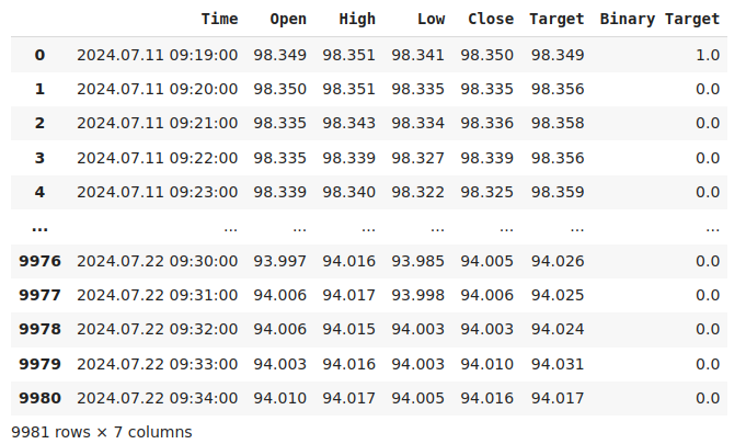

Fig 1: Our current data frame

Exploratory Data Analysis

Let us create scatter-plots to determine if there are any relationships we can observe. Unfortunately, our data appears randomly distributed with no clear separations between up and down moves in the market.

#Lets perform scatter plots
sns.scatterplot(data=nzd_jpy,x=nzd_jpy['Open'], y=nzd_jpy['Close'],hue='Binary Target')

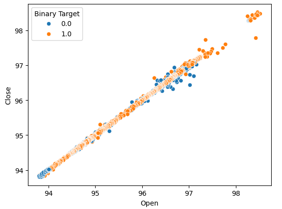
Fig 2: A scatter-plot of the Open and Close price

We thought of creating box plots to summarize all the instances whereby price either rose or fell. We believed that there could potentially be differences between the distribution of data in these 2 possible targets. Regrettably, our box-plots shows that there is hardly any difference between the distribution of data in the two possible outcomes.

#Let's create categorical box plots
sns.catplot(data=nzd_jpy,x='Binary Target',y='Close',kind='box')

Fig 3: A box-plot summarizing all the instances whereby price levels fell (0) or rose (1)

We can also decompose the time-series data into 3 components:

1. Trend
2. Seasonal
   
3. Residual
   

 The trend component represents the average long-term movement of price levels. The seasonal component, accounts for cyclical patterns that are observed repeatedly in the data, while the residual components are the remainder of whatever could not be explained by the previous 2 components. Since we are using M1 data on the NZDJPY pair, we set our period to 1440, or in other words the average performance in price over 1 complete day. We can observe a very clear and strong down-trend in the data even before performing the decomposition. However, by subtracting the trend from the original data, we can now clearly observe the seasonal effects in the data.

#Time series decomposition
import statsmodels.api as sm
nzd_jpy_decomposition = sm.tsa.seasonal_decompose(nzd_jpy['Close'],period=1440,model='additive')
fig = nzd_jpy_decomposition.plot()

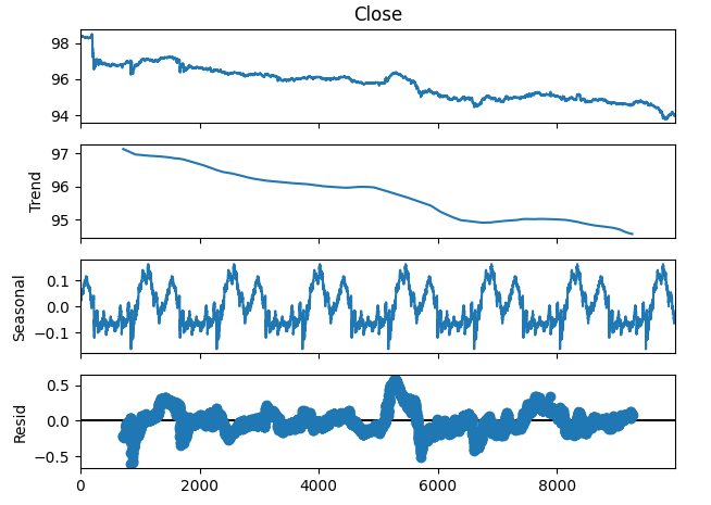
Fig 4: Time-series decomposition of our data

Some effects may be hidden in higher dimensions. Creating 3D scatter-plots of our data, may allows us to unveil effects hidden beyond our scope with a 2D scatter-plot. Unfortunately, this dataset was not one of those cases. Our data is sill quite challenging to separate, and does not display any discernable relationships.

#Let's also perform 3D plots
#Visualizing our data in 3D

import matplotlib.pyplot as plt

fig = plt.figure(figsize=(7,7))
ax = fig.add_subplot(111,projection='3d')
colors = ['blue' if movement == 0 else 'red' for movement in nzd_jpy.loc[:,"Binary Target"]]
ax.scatter(nzd_jpy.loc[:,"Low"],nzd_jpy.loc[:,"High"],nzd_jpy.loc[:,"Close"],c=colors)

ax.set_xlabel('NZDJPY Low')
ax.set_ylabel('NZDJPY High')
ax.set_zlabel('NZDJPY Close')

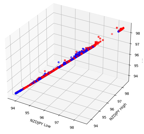
Fig 5: Visualizing our 3D scatter-plot

Preparing To Model The Data

Before we can start modeling our data, we need to first standardize and scale the data. Load the libraries we need.

#Let's prepare the data for modelling
from sklearn.preprocessing import RobustScaler

Scale the data.

#Scale the data
X = pd.DataFrame(RobustScaler().fit_transform(nzd_jpy.loc[:,['Close']]),columns=['Close'])
residuals_X = pd.DataFrame(RobustScaler().fit_transform(nzd_jpy.loc[:,['Open','High','Low']]),columns=['Open','High','Low'])
y = nzd_jpy.loc[:,'Target']

Model Selection

Let us load the libraries we need to model the data.

#Cross validating the models
from sklearn.model_selection import cross_val_score,train_test_split
from sklearn.linear_model import Lasso,LinearRegression,Ridge,ElasticNet,SGDRegressor,HuberRegressor
from sklearn.ensemble import RandomForestRegressor,GradientBoostingRegressor,AdaBoostRegressor,ExtraTreesRegressor,BaggingRegressor
from sklearn.svm import LinearSVR
from sklearn.neighbors import KNeighborsRegressor
from sklearn.tree import DecisionTreeRegressor
from sklearn.neural_network import MLPRegressor

Now partition the data into 2 halves.

#Create train-test splits
train_X,test_X,train_y,test_y = train_test_split(nzd_jpy.loc[:,['Close']],y,test_size=0.5,shuffle=False)
residuals_train_X,residuals_test_X,residuals_train_y,residuals_test_y = train_test_split(nzd_jpy.loc[:,['Open','High','Low']],y,test_size=0.5,shuffle=False)

Store the models in a list and create a data frame to store our validation error levels.

#Store the models
models = [
    Lasso(),
    LinearRegression(),
    Ridge(),
    ElasticNet(),
    SGDRegressor(),
    HuberRegressor(),
    RandomForestRegressor(),
    GradientBoostingRegressor(),
    AdaBoostRegressor(),
    ExtraTreesRegressor(),
    BaggingRegressor(),
    LinearSVR(),
    KNeighborsRegressor(),
    DecisionTreeRegressor(),
    MLPRegressor(),
]

#Store the names of the models
model_names = [
    'Lasso',
    'Linear Regression',
    'Ridge',
    'Elastic Net',
    'SGD Regressor',
    'Huber Regressor',
    'Random Forest Regressor',
    'Gradient Boosting Regressor',
    'Ada Boost Regressor',
    'Extra Trees Regressor',
    'Bagging Regressor',
    'Linear SVR',
    'K Neighbors Regressor',
    'Decision Tree Regressor',
    'MLP Regressor',
]

#Create a dataframe to store our cv error
cv_error = pd.DataFrame(columns=model_names,index=np.arange(0,5))

Cross validate each model.

#Cross validate each model
for model in models:
  cv_score = cross_val_score(model,X,y,cv=5,n_jobs=-1,scoring='neg_mean_squared_error')
  for i in np.arange(0,5):
    index = models.index(model)
    cv_error.iloc[i,index] = cv_score[i]

Visualizing the results.

cv_error

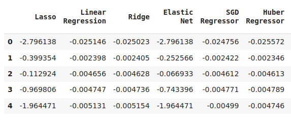
Fig 6: Some of our error levels when forecasting the future close price of the NZDJPY

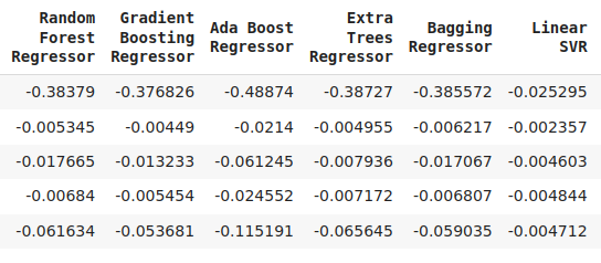
Fig 7: A continuation of our error levels

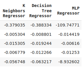
Fig 8: Our final model error levels

We can plot our performance levels across all 5 folds. Our neural network's poor performance was alarming, when we visualized the data in this format. It would probably stand to benefit a lot from parameter-tuning.

cv_error.plot()

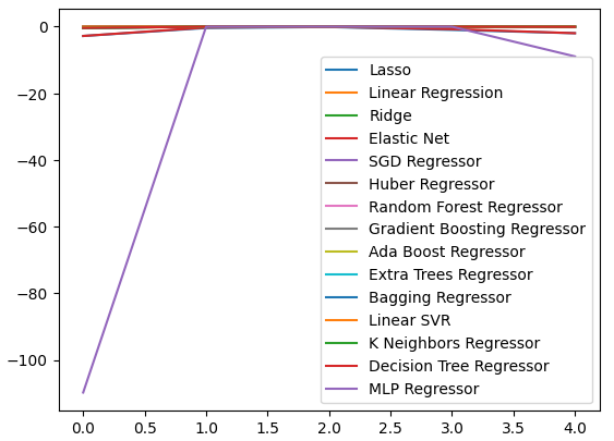
Fig 9: Visualizing our error levels

Box-plots help us summarize a lot of information in a single plot. For example, in our plots below, we can clearly see how poorly the DNN performed on this task. It is the last model on the right, and it is displaying a lot more variance in its performance than the other models.

sns.boxplot(cv_error)

Fig 10: Visualizing our errors as box-plots

We can identify the best performing model as the model with the lowest mean error levels.

#Our mean validation error
cv_error.mean()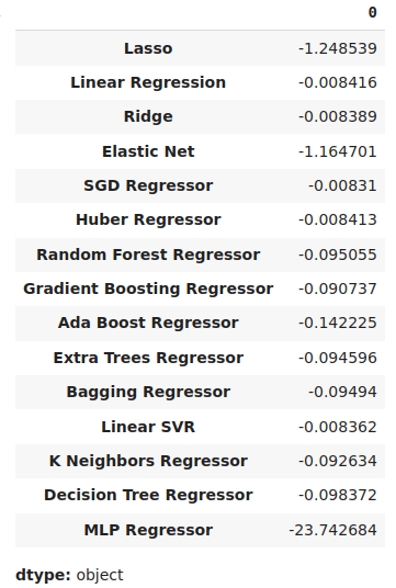

Fig 11: Visualizing our mean error levels

Feature Importance

Feature importance algorithms help us understand whether our model has learned meaningful associations, or if the model has learned relationships we may have not known about. First, let us import the libraries we need.

#Feature importance
from sklearn.feature_selection import mutual_info_regression,RFE

We will begin by calculating mutual information (MI) scores. MI informs us about the potential each predictor posses, to help us predict the target. Lastly, MI is measured on a logarithmic scale. Therefore, MI scores above 3 are rarely seen in practice.

mi_score = pd.DataFrame(mutual_info_regression(X,y),columns=['MI Score'],index=X.columns)

Plotting our MI scores clealy shows us the the High price appears to have the most potential to predict the future close price of the NZDJPY.

mi_score.plot()

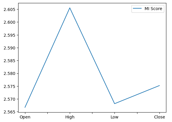
Fig 12: Plotting our MI scores

The RFE algorithm is similarly as straightforward to use as almost any object from the scikit-learn library. We simply create an instance of the class, and fit it to the data, before we can assess the feature importance levels it attributes to each predictor. Our RFE algorithm believed that all the predictors were equally important to predict the NZDJPY close price.

#Select the best features
rfe = RFE(model, n_features_to_select=5, step=1)
rfe = rfe.fit(X, y)
rfe.ranking_

array([1, 1, 1, 1])

Parameter Tuning

Let us now extract as much performance from our SGD Regressor model as we can. We will perform a randomized search over a sample of the parameter space of the model. Let us first import the libraries we need.

#Parameter tuning
from sklearn.model_selection import RandomizedSearchCV

Create an instance of the default model.

#Initialize the model
model = SGDRegressor()

Create a tuner object and specify the possible parameter values we would like to sample.

#Define the tuner
tuner = RandomizedSearchCV(
        model,
        {
        "loss" : ['squared_error', 'huber', 'epsilon_insensitive','squared_epsilon_insensitive'],
        "penalty":['l2','l1', 'elasticnet', None],
        "alpha":[0.1,0.01,0.001,0.0001,0.00001,0.00001,0.0000001,10,100,1000,10000,100000],
        "tol":[0.1,0.01,0.001,0.0001,0.00001,0.000001,0.0000001],
        "fit_intercept": [True,False],
        "early_stopping": [True,False],
        "learning_rate":['constant','optimal','adaptive','invscaling'],
        "shuffle": [True,False]
        },
        n_iter=100,
        cv=5,
        n_jobs=-1,
        scoring="neg_mean_squared_error"
)

Fit the tuner object.

#Fit the tuner
tuner.fit(train_X,train_y)

The best parameters we found.

#Our best parameters
tuner.best_params_

{'tol': 0.001,
 'shuffle': False,
 'penalty': 'elasticnet',
 'loss': 'huber',
 'learning_rate': 'adaptive',
 'fit_intercept': True,
 'early_stopping': True,
 'alpha': 1e-05}

Testing For Overfitting

We can detect overfitting if we observe correlation in the residuals of the model. If a model has learned effectively, its residuals should be random white noise, indicating there is no predictable pattern in the errors being made by our model. However, a model that demonstrates autocorrelation in its residuals may be a cause for concern. It may signal that the regression we have performed is spurious, or that we have selected an inappropriate model for our task.To get started, we need to capture the residuals of our customized model.

#Model validation
model = SGDRegressor(
    tol             = tuner.best_params_['tol'],
    shuffle         = tuner.best_params_['shuffle'],
    penalty         = tuner.best_params_['penalty'],
    loss            = tuner.best_params_['loss'],
    learning_rate   = tuner.best_params_['learning_rate'],
    alpha           = tuner.best_params_['alpha'],
    fit_intercept   = tuner.best_params_['fit_intercept'],
    early_stopping  = tuner.best_params_['early_stopping']
)
model.fit(train_X,train_y)
residuals = test_y - model.predict(test_X)

We can visualize our model's residuals in a plot. Unfortunately, we can clearly see there is autocorrelation in the model’s residuals. In otherwords, whenever the residuals fall, they tend to continue falling, and when the residuals rise, they tend to continue rising. This means that the residuals future values, may have a relationship with its previous values, a tell-tale sign that our model may not have learned effectively, even after performing parameter tuning!

#Plot the residuals
residuals.plot()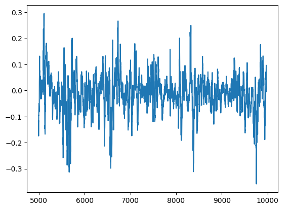

Fig 13: Our model residuals

There are more robust tests for auto-correlation, for example we can create an auto-correlation (ACF) plot. The ACF plot will have spikes at each possible lag value. The height of each spike represents the levels of correlation the time-series data has with its lagged value. There is also a blue cone like structure in the background of our plot, the blue cone represents our confidence intervals. Any correlation levels beyond the confidence interval, are considered statistically significant.

#The residuals appear to have autocorrelation
from statsmodels.graphics.tsaplots import plot_acf
fig = plot_acf(residuals)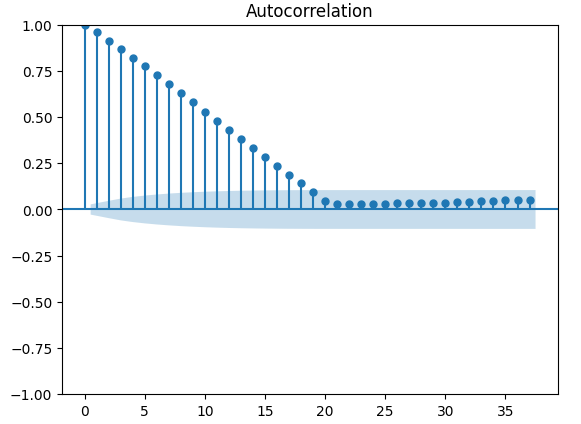

Fig 14: The auto-correlation of our model residuals

This is not a good sign, hopefully we may be able to alleviate this by training our DNN to correct our first model. Let us record our SGD Regresosr’s error’s on the training data and then on the test data. Note, we will not fit the model on the test data at this point, we will only measure its error levels.

#Prepare the residuals for our second model
model = SGDRegressor(tol= 0.001,
 shuffle=False,
 penalty= 'elasticnet',
 loss= 'huber',
 learning_rate='adaptive',
 fit_intercept= True,
 early_stopping= True,
 alpha= 1e-05)

#Store the model residuals
model.fit(train_X,train_y)
residuals_train_y = train_y - model.predict(train_X)
residuals_test_y = test_y - model.predict(test_X)

We will now cross validate out models on predicting the error levels of the SGD Regressor.

#Cross validate each model
for model in models:
  cv_score = cross_val_score(model,residuals_train_X,residuals_train_y,cv=5,n_jobs=-1,scoring='neg_mean_squared_error')
  for i in np.arange(0,5):
    index = models.index(model)
    cv_error.iloc[i,index] = cv_score[i]

Let us visualize the validation error.

#Cross validaton error levels
cv_error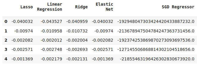

Fig 15: Some of model validation error levels when forecasting our first model's error levels

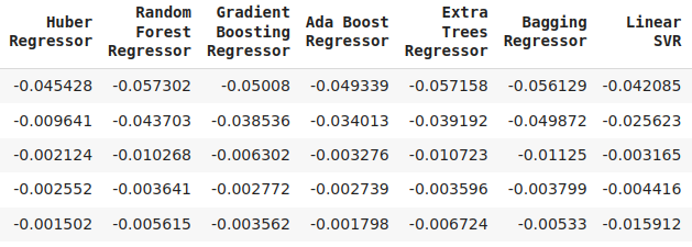
Fig 16: A continuation of our validation error levels

We can view our average error levels in descending order to quickly identify our best performing model.

#Store the model's performance
cv_error.mean().sort_values(ascending=False)

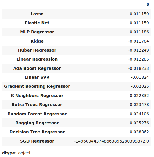
Fig 17: Our mean validation error levels clearly show the Lasso is the best performing model we have

Our box-plots show just how poorly the SGD Regressor performed when trying to predict its own error levels.

sns.boxplot(cv_error)

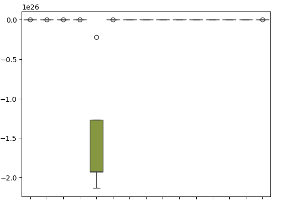
Fig 18: Box-plots of our validation error when forecasting our model's residuals

We can also create line-plots to visualize our data.

cv_error.plot()

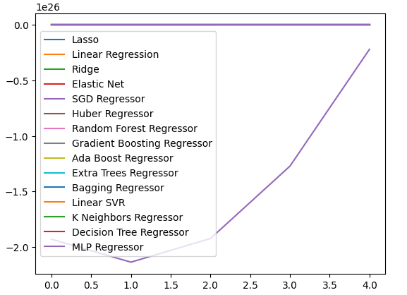
Fig 19: Visualizing our error levels an line plots

Parameter Tuning Our Deep Neural Network

Let us now prepare to tune the parameters of our DNN Regressor, first we will define the tuner object and a sample of the parameter space we wish to search.

#Let's tune the model
#Reinitialize the model

model = MLPRegressor()

#Define the tuner

tuner = RandomizedSearchCV(
        model,
        {
                "activation":["relu","tanh","logistic","identity"],
                "solver":["adam","sgd","lbfgs"],
                "alpha":[0.1,0.01,0.001,0.00001,0.000001],
                "learning_rate": ["constant","invscaling","adaptive"],
                "learning_rate_init":[0.1,0.01,0.001,0.0001,0.000001,0.0000001],
                "power_t":[0.1,0.5,0.9,0.01,0.001,0.0001],
                "shuffle":[True,False],
                "tol":[0.1,0.01,0.001,0.0001,0.00001],
                "hidden_layer_sizes":[(10,20),(100,200),(30,200,40),(5,20,6)],
                "max_iter":[10,50,100,200,300],
                "early_stopping":[True,False]
        },
        n_iter=100,
        cv=5,
        n_jobs=-1,
        scoring="neg_mean_squared_error"
)

Now we will fit the tuner object.

#Fit the tuner
tuner.fit(residuals_train_X,residuals_train_y)

Finally we can see the best parameters we found.

#The best parameters we found
tuner.best_params_

{'tol': 0.0001,
 'solver': 'lbfgs',
 'shuffle': False,
 'power_t': 0.5,
 'max_iter': 300,
 'learning_rate_init': 0.01,
 'learning_rate': 'constant',
 'hidden_layer_sizes': (30, 200, 40),
 'early_stopping': False,
 'alpha': 1e-05,
 'activation': 'identity'}

Deeper Parameter Tuning

Let us now test to see if we cannot find even better parameters still, since we do not necessarily know where the best input values may lie, we will attempt to perform unconstrained global optimization using the limited memory L-BFGS-B algorithm in the SciPy library. The L-BFGS-B algorithm can be effectively used for global optimization problems. The numerical solver itself is implemented in Fortran code, and the SciPy library provides a thin wrapper for easily interfacing with the routine. We will start, by importing the libraries we need.

Fig 20: The developers of the original BFGS algorithm, from left to right: Broyden, Fletcher, Goldfarb and Shanno

#Deeper optimization
from scipy.optimize import minimize

Now we will define the objective function to be minimized, we want to minimize the training error of our DNN Regressor. We will fix all other input parameters of the model since our SciPy minimizers can only handle continuous optimization problems.

#Define the objective function
def objective(x):
    #Create a dataframe to store our accuracy
    cv_error = pd.DataFrame(index = np.arange(0,5),columns=["Current Error"])
    #The parameter x represents a new value for our neural network's settings
    #In order to find optimal settings, we will perform 10 fold cross validation using the new setting
    #And return the average RMSE from all 10 tests
    #We will first turn the model's Alpha parameter, which controls the amount of L2 regularization
    MLPRegressor(hidden_layer_sizes=(20,5),activation='identity',learning_rate='adaptive',solver='lbfgs',shuffle=True,alpha=x[0],tol=x[1])
    model = MLPRegressor(
    tol                 = x[0],
    solver              = tuner.best_params_['solver'],
    power_t             = x[1],
    max_iter            = tuner.best_params_['max_iter'],
    learning_rate       = tuner.best_params_['learning_rate'],
    learning_rate_init  = x[2],
    hidden_layer_sizes  = tuner.best_params_['hidden_layer_sizes'],
    alpha               = x[3],
    early_stopping      = tuner.best_params_['early_stopping'],
    activation          = tuner.best_params_['activation'],
    )
    #Cross validate the model
    cv_score = cross_val_score(model,residuals_train_X,residuals_train_y,cv=5,n_jobs=-1,scoring='neg_mean_squared_error')
    for i in np.arange(0,5):
      cv_error.iloc[i,0] = cv_score[i]
    #Return the Mean CV RMSE
    return(cv_error.iloc[:,0].mean())

We shall define the starting point of our optimization procedure by the best parameters we found from our random search. We will also pass constraints for our optimization procedure, we will force all values to be positive and furthermore we will allow all values in the range of 10 to the power -100 until 10 to the power 100. This is a very large domain, and hopefully it will contain the optimal parameters we are looking for.

#Define the starting point
pt = [tuner.best_params_['tol'],tuner.best_params_['power_t'],tuner.best_params_['learning_rate_init'],tuner.best_params_['alpha']]
bnds = ((10.0 ** -100,10.0 ** 100),
        (10.0 ** -100,10.0 ** 100),
        (10.0 ** -100,10.0 ** 100),
        (10.0 ** -100,10.0 ** 100))

Searching for the best parameters.

#Searching deeper for better parameters
result = minimize(objective,pt,method="L-BFGS-B",bounds=bnds)

Our optimization results.

result

message: CONVERGENCE: REL_REDUCTION_OF_F_<=_FACTR*EPSMCH
  success: True
   status: 0
      fun: -0.01143352283130129
        x: [ 1.000e-04  5.000e-01  1.000e-02  1.000e-05]
      nit: 2
      jac: [-1.388e+04 -4.657e+04  5.625e+04 -1.033e+04]
     nfev: 120
     njev: 24
 hess_inv: <4x4 LbfgsInvHessProduct with dtype=float64>

Testing For Overfitting

Let us now test for overfitting. This time around, we will compare our 2 models, against the performance of the default DNN Regressor. Let us instantiate instances of each DNN Regressor we wish to test.

#Model validation
default_model = MLPRegressor()

customized_model = MLPRegressor(
    tol                 = tuner.best_params_['tol'],
    solver              = tuner.best_params_['solver'],
    power_t             = tuner.best_params_['power_t'],
    max_iter            = tuner.best_params_['max_iter'],
    learning_rate       = tuner.best_params_['learning_rate'],
    learning_rate_init  = tuner.best_params_['learning_rate_init'],
    hidden_layer_sizes  = tuner.best_params_['hidden_layer_sizes'],
    alpha               = tuner.best_params_['alpha'],
    early_stopping      = tuner.best_params_['early_stopping'],
    activation          = tuner.best_params_['activation'],
)

lbfgs_customized_model = MLPRegressor(
    tol                 = result.x[0],
    solver              = tuner.best_params_['solver'],
    power_t             = result.x[1],
    max_iter            = tuner.best_params_['max_iter'],
    learning_rate       = tuner.best_params_['learning_rate'],
    learning_rate_init  = result.x[2],
    hidden_layer_sizes  = tuner.best_params_['hidden_layer_sizes'],
    alpha               = result.x[3],
    early_stopping      = tuner.best_params_['early_stopping'],
    activation          = tuner.best_params_['activation'],
)

Now we will create a list of models and also create a data frame to store out validation error levels.

models = [default_model,customized_model,lbfgs_customized_model]
cv_error = pd.DataFrame(index=np.arange(0,5),columns=['Default NN','Random Search NN','L-BFGS-B NN'])

Cross-validating each model.

#Cross validate the model
for model in models:
  model.fit(residuals_train_X,residuals_train_y)
  cv_score = cross_val_score(model,residuals_test_X,residuals_test_y,cv=5,n_jobs=-1,scoring='neg_mean_squared_error')
  for i in np.arange(0,5):
    index = models.index(model)
    cv_error.iloc[i,index] = cv_score[i]

Our cross-validation error.

cv_error

Default NN	Random Search NN	L-BFGS-B NN
-0.007735	-0.007708	-0.007692
-0.00635	-0.006344	-0.006329
-0.003307	-0.003265	-0.00328
0.005225	-0.004803	-0.004761
-0.004469	-0.004447	-0.004492

Now let us analyze our average error levels.

cv_error.mean().sort_values(ascending=False)

Model	Validation Error
L-BFGS-B NN	-0.005311
Random Search NN	-0.005313
Default NN	-0.005417

As we can see, our model's were all performing within the same range. However, our customized models were clearly providing us with lower error levels on average. Unfortunately, the variance displayed by our models is almost the same across the board, this is shown to us by our box-plots. The variance levels help us determine the model's level of skill,

sns.boxplot(cv_error)

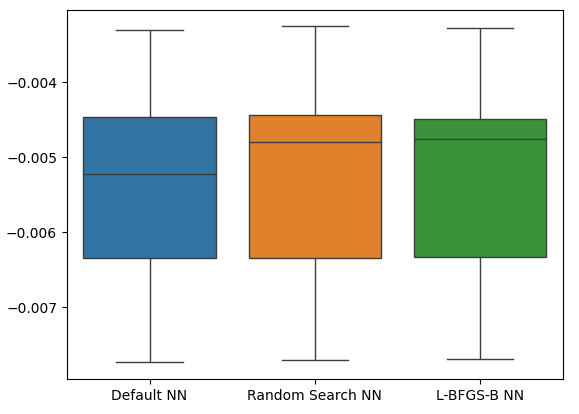
Fig 21: Our validation error levels on the held out data

Let us now see if our ensemble approach is better than just using a single model to forecast price levels. We will first prepare the models we need.

#Now that we have come this far, let's see if our ensemble approach is worth the trouble
baseline = LinearRegression()
default_nn = MLPRegressor()

#The SGD Regressor will predict the future price
sgd_regressor = SGDRegressor(tol= 0.001,
 shuffle=False,
 penalty= 'elasticnet',
 loss= 'huber',
 learning_rate='adaptive',
 fit_intercept= True,
 early_stopping= True,
 alpha= 1e-05)

#The deep neural network will predict the error in the SGDRegressor's prediction
lbfgs_customized_model = MLPRegressor(
    tol                 = result.x[0],
    solver              = tuner.best_params_['solver'],
    power_t             = result.x[1],
    max_iter            = tuner.best_params_['max_iter'],
    learning_rate       = tuner.best_params_['learning_rate'],
    learning_rate_init  = result.x[2],
    hidden_layer_sizes  = tuner.best_params_['hidden_layer_sizes'],
    alpha               = result.x[3],
    early_stopping      = tuner.best_params_['early_stopping'],
    activation          = tuner.best_params_['activation'],
)

Fitting the model's on the training set.

#Fit the models on the train set
baseline.fit(train_X.loc[:,['Close']],train_y)
default_nn.fit(train_X.loc[:,['Close']],train_y)
sgd_regressor.fit(train_X.loc[:,['Close']],train_y)
lbfgs_customized_model.fit(residuals_train_X.loc[:,['Open','High','Low']],residuals_train_y)

Store the models in a list.

#Store the models in a list
models = [baseline,default_nn,sgd_regressor,lbfgs_customized_model]

Creating a data-frame to store our error levels.

#Create a dataframe to store our error
ensemble_error = pd.DataFrame(index=np.arange(0,5),columns=['Baseline','Default NN','SGD','Customized NN'])

Importing the libraries we need.

from sklearn.model_selection import TimeSeriesSplit
from sklearn.metrics import mean_squared_error

Create the time-series split object.

#Create the time-series object
tscv = TimeSeriesSplit(n_splits=5,gap=20)

We need to reset the indexes of our data.

#Reset the indexes so we can perform cross validation
test_y = test_y.reset_index()
residuals_test_y = residuals_test_y.reset_index()

test_X = test_X.reset_index()
residuals_test_X = residuals_test_X.reset_index()

Now we will perform time-series cross-validation. Note that the model predicting the residuals needs to be trained separately from the other models that are simply predicting the future close price.

#Cross validate the models
for j in np.arange(0,4):
  model = models[j]
  for i,(train,test) in enumerate(tscv.split(test_X)):
    #The model predicting the residuals
    if(j == 3):
      model.fit(residuals_test_X.loc[train[0]:train[-1],['Open','High','Low']],residuals_test_y.loc[train[0]:train[-1],'Target'])
      #Measure the loss
      ensemble_error.iloc[i,j] = mean_squared_error(residuals_test_y.loc[test[0]:test[-1],'Target' ], model.predict(residuals_test_X.loc[test[0]:test[-1],['Open','High','Low']]))

    elif(j <= 2):
      #Fit the model
      model.fit(test_X.loc[train[0]:train[-1],['Close']],test_y.loc[train[0]:train[-1],'Target'])
      #Measure the loss
      ensemble_error.iloc[i,j] = mean_squared_error(test_y.loc[test[0]:test[-1],'Target' ],model.predict(test_X.loc[test[0]:test[-1],['Close']]))

Now let us analyze our validation error levels. Unfortunately, we failed to outperform the performance of a simple linear regression model, indicating that our model may be too sensitive to the variance of the data. The good news is that we out performed our default DNN Regressor.

ensemble_error.mean().sort_values(ascending=True)

Models	Validation Error
Baseline	0.004784
Customized L-BFGS-B NN	0.004891
SGD	0.005937
Default NN	35.35851

Exporting To ONNX Format

Open Neural Network Exchange (ONNX) is an open-source protocol for building and deploying machine learning models in a language agnostic manner. ONNX allows us to easily integrate our scikit-learn models into our Expert Advisors by relying on the MQL5 API support for ONNX. First, we will import the libraries we need.

#Prepare to export to ONNX
import onnx
import netron
from   skl2onnx import convert_sklearn
from   skl2onnx.common.data_types import FloatTensorType

Now let us fit the models on all the data we have available.

#Fit the SGD model on all the data we have
close_model = SGDRegressor(tol= 0.001,
 shuffle=False,
 penalty= 'elasticnet',
 loss= 'huber',
 learning_rate='adaptive',
 fit_intercept= True,
 early_stopping= True,
 alpha= 1e-05)

close_model.fit(nzd_jpy.loc[:,['Close']],nzd_jpy.loc[:,'Target'])

Then lastly we will fit our DNN Regressor.

#Fit the deep neural network on all the data we have
residuals_model = MLPRegressor(
 tol=0.0001,
 solver= 'lbfgs',
 shuffle=False,
 power_t= 0.5,
 max_iter= 300,
 learning_rate_init= 0.01,
 learning_rate='constant',
 hidden_layer_sizes=(30, 200, 40),
 early_stopping=False,
 alpha=1e-05,
 activation='identity')

#Fit the model on the residuals
residuals_model.fit(residuals_train_X,residuals_train_y)
residuals_model.fit(residuals_test_X,residuals_test_y)

Let us define the input shapes of our 2 models.

# Define the input type
close_initial_types = [("float_input",FloatTensorType([1,1]))]
residuals_initial_types = [("float_input",FloatTensorType([1,3]))]

We need to create ONNX representations of our models.

# Create the ONNX representation
close_onnx_model = convert_sklearn(close_model,initial_types=close_initial_types,target_opset=12)
residuals_onnx_model = convert_sklearn(residuals_model,initial_types=residuals_initial_types,target_opset=12)

Lastly, we need to store our models in ONNX format.

#Save the ONNX Models
onnx.save_model(close_onnx_model,'close_model.onnx')
onnx.save_model(residuals_onnx_model,'residuals_model.onnx')

Visualizing our ONNX Models

Let us also visualize our models to ensure that they have the input and output shapes we specifeid. We will start by visualizing our DNN Regressor. First, we will import the library we need.

#Import netron
import netron 

Now we will visualize our DNN.

#Visualizing the residuals model
netron.start("/ENTER/YOUR/PATH/residuals_model.onnx")

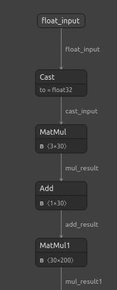
Fig 22: Visualizing our DNN Regressor model

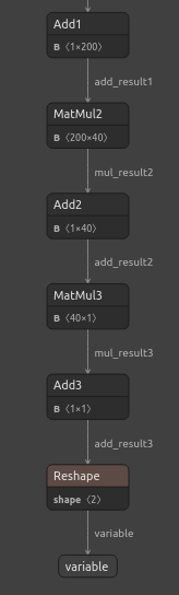
Fig 23: Visualizing our DNN Regressor Model

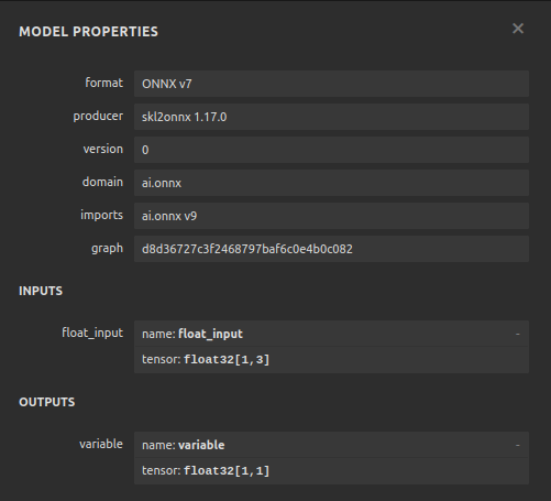
Fig 24: The input and output shape of our DNN regressor meets our expectations

Let us also visualize our SGD Regressor model.

#Visualizing the close model
netron.start("/ENTER/YOUR/PATH/close_model.onnx")

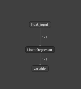
Fig 25: Visualizing our SGD Regressor model

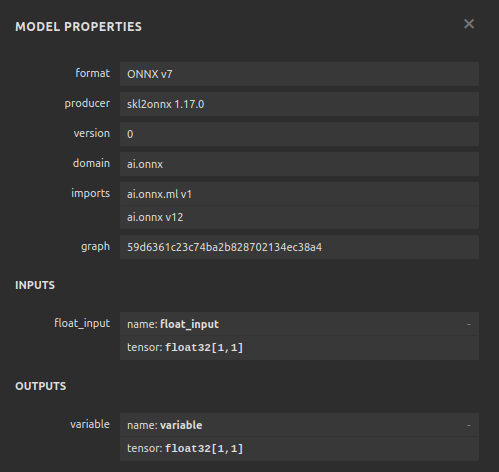
Fig 26: Visualizing our SGD Regressor model

Implementing in MQL5

To start building our AI-powered Expert Advisor, we first need to load the ONNX files we have just created into the application.

//+------------------------------------------------------------------+
//|                                                   NZD JPY AI.mq5 |
//|                                        Gamuchirai Zororo Ndawana |
//|                          https://www.mql5.com/en/gamuchiraindawa |
//+------------------------------------------------------------------+
#property copyright "Gamuchirai Zororo Ndawana"
#property link      "https://www.mql5.com/en/gamuchiraindawa"
#property version   "1.00"

//+------------------------------------------------------------------+
//| Load the ONNX models                                             |
//+------------------------------------------------------------------+
#resource "\\Files\\residuals_model.onnx" as const uchar residuals_onnx_buffer[];
#resource "\\Files\\close_model.onnx" as const uchar close_onnx_buffer[];

Now, we need the trade library to help us open and close our positions.

//+------------------------------------------------------------------+
//| Libraries                                                        |
//+------------------------------------------------------------------+
#include  <Trade/Trade.mqh>
CTrade Trade;

Let us also create global variables that we will use throughout our program.

//+------------------------------------------------------------------+
//| Global variables                                                 |
//+------------------------------------------------------------------+
long residuals_model,close_model;
vectorf residuals_forecast   = vectorf::Zeros(1);
vectorf close_forecast       = vectorf::Zeros(1);
float forecast = 0;
int model_state,system_state;
int counter = 0;
double bid,ask;

In our model's initialization procedure, we will first load our 2 ONNX models, then we will validate that our models are working.

//+------------------------------------------------------------------+
//| Expert initialization function                                   |
//+------------------------------------------------------------------+
int OnInit()
  {
//--- Load the ONNX models
   if(!load_onnx_models())
     {
      return(INIT_FAILED);
     }

//--- Validate the model is working
   model_predict();
   if(forecast == 0)
     {
      Comment("The ONNX models are not working correctly!");
      return(INIT_FAILED);
     }

//--- We managed to load our ONNX models
   return(INIT_SUCCEEDED);
  }

Whenever our model is removed from the chart, we will free up any resoruces we are no longer using.

//+------------------------------------------------------------------+
//| Expert deinitialization function                                 |
//+------------------------------------------------------------------+
void OnDeinit(const int reason)
  {
//--- Free up the resources we no longer need
   release_resorces();
  }

If we receive any new prices, we will first update our market prices. Afterwards, we will fetch a prediction from our model. Once we have a forecast, we will check if we have any positions open. If we have no open positions, we will then follow our model's prediction so long as the price changes on higher time frames permits us to do so. Otherwise, if we allready have an open position, we will first wait for 20 candles to elapse before checking to see if our model is predicting a reversal. Recall that we trained the model to forecast 20 steps into the future, therefore we should allow some time to elapse before checking for a reversal.

//--- If we have no positions, follow the model's forecast
   if(PositionsTotal() == 0)
     {
      //--- Our model is suggesting we should buy
      if(model_state == 1)
        {
         if(iClose(Symbol(),PERIOD_W1,0) > iClose(Symbol(),PERIOD_W1,12))
           {
            Trade.Buy(0.3,Symbol(),ask,0,0,"NZD JPY AI");
            system_state = 1;
           }
        }

      //--- Our model is suggesting we should sell
      if(model_state == -1)
        {
         if(iClose(Symbol(),PERIOD_W1,0) < iClose(Symbol(),PERIOD_W1,12))
           {
            Trade.Sell(0.3,Symbol(),bid,0,0,"NZD JPY AI");
            system_state = -1;
           }
        }
     }

   else
     {
      //--- We want to wait 20 mins before forecating again.
      if(time_stamp != time)
        {
         time_stamp= time;
         counter += 1;
        }

      if((system_state!= model_state) && (counter >= 20))
        {
         Alert("Reversal detected by our AI system, closing all positions");
         Trade.PositionClose(Symbol());
         counter = 0;
        }
     }
  }

Let us define the function to fetch prediction from our models, recall that we have 2 separate models that each need to be called in turn.

//+------------------------------------------------------------------+
//| Fetch a prediction from our models                               |
//+------------------------------------------------------------------+
void model_predict(void)
  {
//--- Define the inputs
   vectorf close_inputs = vectorf::Zeros(1);
   vectorf residuals_inputs = vectorf::Zeros(3);

   close_inputs[0]     = (float) iClose(Symbol(),PERIOD_M1,0);
   residuals_inputs[0] = (float) iOpen(Symbol(),PERIOD_M1,0);
   residuals_inputs[1] = (float) iHigh(Symbol(),PERIOD_M1,0);
   residuals_inputs[2] = (float) iLow(Symbol(),PERIOD_M1,0);

//--- Fetch predictions
   OnnxRun(residuals_model,ONNX_DEFAULT,residuals_inputs,residuals_forecast);
   OnnxRun(close_model,ONNX_DEFAULT,close_inputs,close_forecast);

//--- Our forecast
   forecast = residuals_forecast[0] + close_forecast[0];
   Comment("Model forecast: ",forecast);

//--- Remember the model's prediction
   if(forecast > close_inputs[0])
     {
      model_state = 1;
     }
   else
     {
      model_state = -1;
     }
  }

We also need a function to update our market prices.

//+------------------------------------------------------------------+
//| Update the market data we have                                   |
//+------------------------------------------------------------------+
void update_market_data(void)
  {
   bid = SymbolInfoDouble(Symbol(),SYMBOL_BID);
   ask = SymbolInfoDouble(Symbol(),SYMBOL_ASK);
  }

This function will release the resources we are no longer using.

//+------------------------------------------------------------------+
//| Rlease the resources we no longer need                           |
//+------------------------------------------------------------------+
void release_resorces(void)
  {
   OnnxRelease(residuals_model);
   OnnxRelease(close_model);
   ExpertRemove();
  }

Lastly, this function will prepare our ONNX models from the ONNX buffers we created in the beginning of our application.

//+------------------------------------------------------------------+
//| This function will load our ONNX models                          |
//+------------------------------------------------------------------+
bool load_onnx_models(void)
  {
//--- Load the ONNX models from the buffers we created
   residuals_model = OnnxCreateFromBuffer(residuals_onnx_buffer,ONNX_DEFAULT);
   close_model = OnnxCreateFromBuffer(close_onnx_buffer,ONNX_DEFAULT);

//--- Validate the models
   if((residuals_model == INVALID_HANDLE) || (close_model == INVALID_HANDLE))
     {
      //--- We failed to load the models
      Comment("Failed to create the ONNX models: ",GetLastError());
      return(false);
     }

//--- Set the I/O shapes of the models
   ulong residuals_inputs[] = {1,3};
   ulong close_inputs[]     = {1,1};
   ulong model_output[]     = {1,1};

//---- Validate the I/O shapes
   if((!OnnxSetInputShape(residuals_model,0,residuals_inputs)) || (!OnnxSetInputShape(close_model,0,close_inputs)))
     {
      //--- We failed to set the input shapes
      Comment("Failed to set model input shapes: ",GetLastError());
      return(false);
     }

   if((!OnnxSetOutputShape(residuals_model,0,model_output)) || (!OnnxSetOutputShape(close_model,0,model_output)))
     {
      //--- We failed to set the output shapes
      Comment("Failed to set model output shapes: ",GetLastError());
      return(false);
     }

//--- Everything went fine
   return(true);
  }
//+------------------------------------------------------------------+

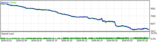
Fig 27: Back testing our Expert Advisor

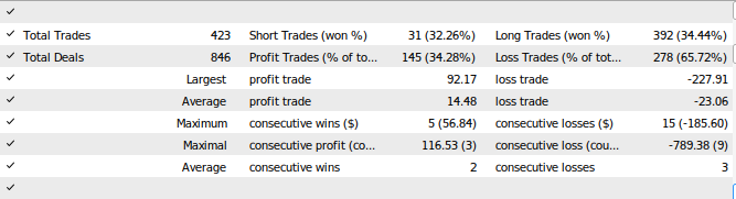
Fig 28: The results of testing our Expert Advisor

Conclusion

In this article, we have demonstrated how we can build self-correcting trading applications. Our conversation highlighted how to analyze your model's residuals to detect for overfitting and bias in your machine learning models. Unfortunately, we detected that our best performing model's residuals were miss-behaved. We could try to remedy this by differencing the time-series data and the target until we no longer observe any autocorrelation in the residuals, however this could also make our model more challenging to interpret. While we cannot guarantee that the points we have raised in this article will generate consistent success, it is definitely worth considering if you are keen on applying AI into your trading strategies. Join us for our next discussion as we will try to remedy the pitfalls we have observed today, while balancing model interpretability.