Markov Chain Monte Carlo Sampling Methods: The HMC Algorithm

Introduction

Bayesian modeling and Markov chain Monte Carlo (MCMC) methods form the basis for solving complex probabilistic problems in machine learning. However, traditional MCMC algorithms based on random walks (such as Metropolis-Hastings) face a fundamental problem in high-dimensional models — the “curse of dimensionality.”

As the number of parameters being estimated increases, these methods are forced to take excessively small steps in order to maintain a reasonable acceptance probability. This results in slow exploration of the space, high autocorrelation in the samples, and, consequently, low performance.

The Hamiltonian Monte Carlo (HMC) algorithm solves this problem by drawing on the principles of Hamiltonian mechanics and information about the gradient of the log density of the target distribution. Instead of taking short, random steps, HMC follows long, directed trajectories, effectively moving toward regions of high probability. Just as in an optimization problem, access to the gradient dramatically speeds up the search. This allows HMC to operate even in high-dimensional spaces where traditional methods fail.

To illustrate how HMC works, a complex test case is used — sampling from a 100-dimensional correlated normal distribution with widely varying variances. The key elements that ensure the robustness and stability of the developed implementation are considered:

• adaptive tuning of the integration step size epsilon and the diagonal mass matrix M,
• MAP estimation using the L-BFGS method to accelerate the warm-up period.

To assess the quality of the samples obtained, comprehensive diagnostics (Rhat, ESS, MCSE, Mean, SD, quantiles) and real-time process monitoring have been implemented.

Dynamical Basis of HMC

HMC is a gradient-based MCMC method with auxiliary variables that originated in physics. It is based on Hamiltonian mechanics, which makes it possible to construct directed trajectories in parameter space while avoiding chaotic random walks.

The main components of HMC are:

• potential energy E(z): equals the negative logarithm of the target probability density: E(z) = - log p(z)
• auxiliary momentum r: it is typically drawn from a simple distribution, usually a multivariate normal distribution r ∼ N(0, M), where M is the mass matrix
• kinetic energy K(r): equals the negative logarithm of the momentum distribution
• total energy (Hamiltonian) H(z, r): represents the total energy of the system

H(z, r) = E(z) + K(r)

The motion of the HMC chain occurs in what is known as phase space, which is the joint space of the parameters z (position) and the auxiliary momentum r.

The Hamiltonian dynamics described below produces a deterministic trajectory in this (z, r) space. Motion along this trajectory conserves the total energy (Hamiltonian). This property ensures reversibility and volume preservation in phase space, which is necessary for the correctness of the Monte Carlo algorithm.

The evolution of z(t) and r(t) over time is described by two coupled differential equations of motion:

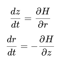
Fig. 1. Hamilton's Equations of Motion

The position equation (dz/dt) determines how quickly and in what direction the position z changes. The rate of change of the position z is expressed in terms of the derivative of the Hamiltonian with respect to the momentum r. Since H(z, r) depends on r only through the kinetic energy

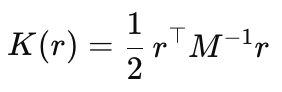
the partial derivative ∂H/∂r is equal to the inverse mass matrix multiplied by the momentum.

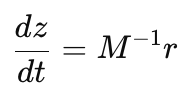
In this context, the matrix M determines the inertia (or “heaviness”) of the parameters. If a parameter has a large mass, its motion slows down. This allows the algorithm to regulate the effective dynamics across different dimensions, ensuring more uniform exploration of the space.

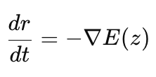
The momentum equation (dr/dt) determines how the momentum r changes at each point in the z space. The rate of change of the momentum r is proportional to the negative gradient of the potential energy, -∇E(z), which is essentially the gradient of the log target density. Thus, this equation describes the force that guides the chain toward increasing target density, pushing the samples toward regions of high probability.

With ideal continuous integration of the Hamiltonian equations, the total energy H(z, r) is conserved along the entire trajectory. This can be seen by writing out the total derivative of the Hamiltonian with respect to time:

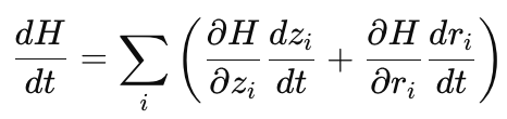
Now, if we substitute the equations of motion into this formula, we obtain the following expression:

in which the terms cancel each other out and, consequently, the derivative with respect to time is equal to zero. This means that energy remains constant and the system cannot transition from one energy level to another. If the total energy at the beginning of the trajectory is, say, 10, then it will also be 10 at the end of the trajectory (in an ideal case). The chain of parameter values z moves, but only within a single energy surface — the set of points (z, r) where H(z, r) = 10. Without changing the energy level, the chain samples only a small portion of the target distribution.

To address the problem of getting stuck on a single energy surface, HMC randomly selects a new momentum vector r from the normal distribution p(r) at the beginning of each iteration. This changes the kinetic energy, and consequently the total energy H also changes. The chain jumps to a new energy surface and continues its motion there. Thus, step by step, it moves between energy levels — and, consequently, all regions of the parameter space z that correspond to the target distribution.

Numerical Integration and the “Leapfrog” Method

In practice, the continuous Hamiltonian equations are solved numerically. Conventional methods, such as Euler's method, introduce errors that violate energy conservation, distort the phase-space volume, and make the trajectory irreversible, which is unacceptable for MCMC. That is why HMC uses a special “leapfrog” integration method. Its advantage is that it exactly preserves phase-space volume, is fully reversible, and offers high accuracy, ensuring that the samples remain unbiased even for long trajectories.

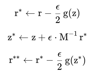
Fig. 2. Schematic of a single Leapfrog step: alternating momentum half-steps and a full position step

A single full step of size ϵ consists of three stages that alternate between updating momentum and position. First, the momentum r is updated by half a step, ϵ/2, using the negative gradient of the potential energy at the current point z. Next, the position z is shifted by a full step ϵ, using the updated momentum scaled by the inverse of the mass matrix M. After that, we compute the new gradient of the potential energy, g, at the new position z and perform the second half-step for the momentum, again with ϵ/2. This sequence minimizes error and preserves the symmetry of the trajectory.

//--- Leapfrog steps
         for(int l = 0; l < num_leapfrog; l++)
           {
            r = r - (epsilon / 2.0) * g_new; // Half-step for the momentum        
            z = z + epsilon * M_inv * r;     // Full step for position z, taking M^-1 into account
            E(z, g_new, e, log_pdf, false);  // Calculate the new gradient
            r = r - (epsilon / 2.0) * g_new; // Another half-step for the momentum
           }

However, even the Leapfrog method does not conserve total energy perfectly; small numerical errors still accumulate over time. Therefore, deviations from energy conservation are corrected using the Metropolis-Hastings acceptance criterion. After constructing the trajectory (a series of Leapfrog steps), we obtain a candidate state (z∗, r∗) and accept it with a probability based on the difference in total energy H before and after integration:

min(1, exp { H(z, r) - H(z*, r*) })

For numerical stability, this condition is checked in an equivalent logarithmic form. A candidate is accepted if the natural logarithm of a uniformly distributed random number u ∼ U(0,1) is less than the difference between the old and new energies:

ln(u) < H(z, r) − H(z*, r*)

If the energy has remained virtually unchanged (H(z, r) ≈ H(z*, r*)), the difference is close to zero, and the acceptance probability will be close to 100%. If the integration error is large, the candidate is likely to be rejected. Thus, the Metropolis step corrects the inaccuracies of the Leapfrog method, ensuring that all samples remain valid and unbiased.

MAP Estimation

Before proceeding to the main sampling phase, it is helpful to move the starting point of the chain to a high-probability region. This approach significantly shortens the warm-up (burn-in) period, since it is best to begin sampling from a high-density region.

The MAP (maximum a posteriori) estimate is the point z at which the target probability density p(z) reaches its maximum. Because the potential energy E(z) is defined as the negative logarithm of the probability density, MAP estimation reduces to the equivalent problem of minimizing the potential energy.

To find the MAP estimate in our code, we use the L-BFGS optimization method (Alglib library). The MAP estimate obtained after successful minimization becomes the starting point for the main sampling phase or for the mass matrix tuning phase. Thus, MAP estimation ensures that HMC starts from the most promising region of the parameter space.

HMC Parameter Tuning

To ensure high efficiency of HMC in real-world problems, especially in high-dimensional spaces, two key parameters must be tuned adaptively: the integration step size epsilon and the mass matrix M.

Step Size Adaptation

The integration step size epsilon (the leapfrog step size) is a key parameter that determines the accuracy of the numerical solution of the Hamiltonian equations:

• a step size that is too large leads to a significant integration error, a violation of energy conservation, and, as a result, a low acceptance probability,
• If epsilon is too small, an excessively large number of steps L is required to construct a single trajectory, which makes sampling unreasonably slow.

The goal of adaptation is to maintain the actual acceptance probability within the optimal range (typically 65%–95%). In our algorithm, this is achieved using an exponential moving average (EMA) of the actual acceptance probability. The EMA smooths out short-term fluctuations, allowing the algorithm to respond smoothly to changes in the probability landscape:

• if the acceptance EMA is above the target value (the integration accuracy is too high), epsilon is increased slightly;
• if the acceptance EMA is below the target value (many rejections), epsilon is reduced to decrease the integration error and increase the chance of acceptance.

This approach ensures that HMC uses the largest possible step size epsilon, allowing it to move quickly through the space while maintaining a high and stable acceptance probability.

Mass Matrix Adaptation

Although step size adaptation makes it possible to control the total length of the trajectory, it does not solve the scaling problem in a heteroscedastic space, i.e., one in which different dimensions have substantially different variances. If the target distribution is highly elongated (for example, the variance along z1 is 100 and along z2 is 0.01), a single step size epsilon cannot be optimal for both axes at once: it will be too small for the wide z1 axis and too large for the narrow z2 axis.

This is exactly where the mass matrix M comes into play. It acts as a metric on the space, rescaling the coordinates so that the sampler sees the distribution as isotropic — that is, close to spherical. This is achieved because the mass matrix controls the chain's velocity along each axis separately. Axes with low variance (narrow directions) are assigned a larger mass, which slows down the motion and prevents abrupt jumps over the density peak. Conversely, axes with high variance (wide directions) are assigned a small mass, allowing the chain to explore broad regions quickly and reliably.

Ideally, the mass matrix should be proportional to the inverse covariance matrix of the target distribution. In that case, an elongated, correlated, or heteroscedastic distribution is transformed into a space where all directions have approximately the same scale. As a result, it is now possible to use a single shared step size epsilon that is appropriate for all axes, without having to sacrifice accuracy for speed — or vice versa. As a result, the overall sampling efficiency increases significantly.

In our HMC implementation, we use two approaches to tuning the diagonal mass matrix:

• a Hessian-based estimate at the maximum a posteriori (MAP) point,
• iterative sampling, which gradually refines the variance estimates based on the accumulated samples

Both methods make it possible to start the main sampling phase with an already well-tuned mass matrix, which significantly speeds up convergence and improves the quality of the samples.

Hessian-based tuning at the MAP point

The most straightforward approach is based on the fact that, near the maximum, the target density p(z) can often be approximated by a multivariate normal distribution. In this case, the covariance matrix Σ of the target distribution is inversely proportional to the Hessian H of the potential energy E(z): Σ = H⁻¹. Since the mass matrix should be proportional to the inverse covariance matrix, we obtain: M ≈ H. Thus, the optimal mass matrix is the Hessian of the potential energy at the MAP point.

Since computing the full Hessian (the matrix of second derivatives) is too computationally expensive, we will compute only its diagonal elements, calculated at the maximum a posteriori (MAP) point. The GetDiagonalHessian function uses the central difference method to approximate these derivatives:

//+------------------------------------------------------------------+
//| Numerically computes the diagonal Hessian of the LogPDF          |
//+------------------------------------------------------------------+
vector  GetDiagonalHessian(LogPDF *log_pdf, const vector &theta)
     {
      // Set the step size h.
      double h = 1e-5;
      
      int n = (int)theta.Size();
      vector Hdiag(n);

      // Calculate fun(theta)
      double funtheta = log_pdf.LogTarget(theta);
      vector theta_h = theta;
      // 4. Calculation of the diagonal elements H_ii
      for(int i = 0; i < n; i++)
        {
         // f(x + 2h*e_i)
         theta_h[i] = theta[i] + 2.0 * h;
         double fun_plus_2h = log_pdf.LogTarget(theta_h);

         // f(x - 2h*e_i)
         theta_h[i] = theta[i] - 2.0 * h;
         double fun_minus_2h = log_pdf.LogTarget(theta_h);

         // Restore x_i
         theta_h[i] = theta[i];

         // Central difference: (f(x+2h) + f(x-2h) - 2f(x)) / (4h^2)
         Hdiag[i] = (fun_plus_2h + fun_minus_2h - 2.0 * funtheta) / (4.0 * h * h);
        }

      return Hdiag;
     }

   //+------------------------------------------------------------------+
   //| Adaptively tunes the mass matrix M based on the LogPDF Hessian   |
   //+------------------------------------------------------------------+
   vector  TuneHessian(LogPDF *log_pdf, const vector &start_point)
     {
      // regularization
      double reg = 1e-3;

      // 1. Compute the negative diagonal Hessian of the LogPDF
      // M = -H
      vector negdiaghessian = -1.0 * GetDiagonalHessian(log_pdf, start_point);

      // 2. Regularization: massvec = max(reg, negdiaghessian).
      int n = (int)negdiaghessian.Size();
      vector massvec(n);
     
      for(int i = 0; i < n; i++)
        {
         if(negdiaghessian[i] < reg)
           {
            // Replace negative or excessively small values with reg
            massvec[i] = reg;
           }
         else
           {
            massvec[i] = negdiaghessian[i];
           }
        }
      return massvec;
     }

However, this method is most effective when the target distribution p(z) is indeed close to a normal distribution. If a distribution has a complex shape (for example, multiple modes), the Hessian calculated at a single point cannot adequately capture that distribution. In that case, the iterative sampling method is more reliable.

Iterative Sampling (Adaptation Based on Sample Variance)

The iterative sampling method is an empirical approach that allows the algorithm to adapt the mass matrix based on the chain's actual behavior. The main idea is to gradually improve the accuracy of the matrix using samples that the chain generates on its own.

The process begins with a small number of samples and an initial mass matrix M. At each iteration, HMC is run to generate N samples of z. Next, the empirical variance Var(z(i)) of these samples is calculated for each coordinate. The mass matrix is updated based on this variance using the following formula:

M(i) = 1 / (Var(z(i)) + λ)

where λ is a small regularization term to prevent division by zero.

To improve the reliability of the variance estimate, the number of samples in each subsequent iteration is increased, and the endpoint of the previous chain is used as the starting point for the next iteration.

//+------------------------------------------------------+
//| Mass matrix tuning using iterative sampling          |
//+------------------------------------------------------+
bool TuneIterativeSampling(
    LogPDF *log_pdf, 
    HMC_Params &params,
    const vector &initial_x, // Starting point for the first iteration
    vector &mass_vec_out,    // Final mass vector
    vector &endpoint_out     // Endpoint of the last chain
    )
{
    ulong n = initial_x.Size();
    
    // Create a copy of the parameters
    HMC_Params current_params = params;    
    current_params.DisableEpsilonAdaptation  = true;
    current_params.burnin   = 0; // During tuning, we do not need a burn-in period or thinning.
    current_params.ThinSize = 1; 
    current_params.num_print = 0; // Disable informational output
    
    // Initial mass vector: M = M_initial * Multiplier
    vector mass_vec = params.mass_vector * params.IterativeSamplingInitialMassMultiplier;
    current_params.mass_vector = mass_vec;   
    int num_samples = params.IterativeSamplingMinSamples;  
    matrix xsmpl_matrix;
    double acceptance_rate = 0.0;
    vector current_start_point = initial_x;
    vector current_endpoint(n); 
    
    PrintFormat("Iterative mass matrix tuning (%d iterations) ", params.IterativeSamplingIterations);
    for (int i = 1; i <= params.IterativeSamplingIterations; i++)
    {
        current_params.num_samples = num_samples;
        
        HMC(current_start_point, xsmpl_matrix, acceptance_rate, log_pdf, current_params, current_endpoint);

        vector variance_vec = xsmpl_matrix.Var(1,1);       
        vector new_mass_vec(n);                 
        new_mass_vec = 1.0 / (variance_vec + params.IterativeSamplingRegularizer);       
        mass_vec = new_mass_vec;
        current_params.mass_vector = mass_vec; // Update M for the next HMC iteration
        PrintFormat("  Iteration %d: Samples=%d ", i, current_params.num_samples);        
        // Increase the sample size
        num_samples = MathMin(num_samples * 2, params.IterativeSamplingMaxSamples);       
        // Set the starting point for the next iteration
        current_start_point = current_endpoint;
    }
    
    // Set the final values
    mass_vec_out = mass_vec; 
    endpoint_out = current_endpoint;   
    params.mass_vector = mass_vec; 

    return true;
}

This approach makes it possible to select optimal parameter scaling that also works for non-Gaussian distributions.

Real-Time Sampling Monitoring

During HMC operation, diagnostic information is written to the log. The logging frequency is controlled by the `num_print` parameter of the `HMC_Params` structure:

• if num_print = 0, output is disabled;
• if `num_print` is a positive integer (for example, 100), information will be output every 100 saved samples after the warm-up period is complete.

Real-time monitoring makes it possible to:

1. Check for stationarity (LOG PDF): verify that the mean log density has stopped increasing and is fluctuating around a stable level. This indicates that the chain has successfully reached the high-probability region and has begun sampling from the target distribution.
2. Monitor step size adaptation (STEP SIZE), which is performed automatically to maintain the target acceptance probability.
3. Monitor the mean acceptance probability (ACC RATIO), which should remain close to the target value specified by the user.
4. Track the number of divergences (DIVERGENT), i.e., trajectories in which the Hamiltonian was not conserved; this often indicates problems with the model or an excessively large step size. Ideally, there should be no divergences.

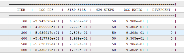
Fig. 3. Example of information output during sampling

MCMC Diagnostic Metrics

The Diagnostics function is responsible for calculating statistics and writing them to the log. It evaluates key metrics across all chains:

• estimate of the mean (Mean)
• standard deviation (SD)
• Monte Carlo standard error (MCSE) — measures the precision with which we can estimate the mean. MCSE = SD / sqrt(ESS). The lower the MCSE, the more accurate our estimate of the mean.

• Quantiles (Q5, Q95)
• Effective Sample Size (ESS) — determines how many independent samples are equivalent, in terms of information content, to the entire MCMC sample. In MCMC, samples are correlated (each sample depends on the previous one), so ESS is less than the actual sample size. The higher the ESS, the lower the autocorrelation and the more useful information there is in the sample.

• The Gelman-Rubin convergence statistic (R-hat) — estimates how well different independent MCMC chains mix and converge to the same target distribution. R-hat values close to 1 (typically < 1.1) indicate satisfactory convergence, with between-chain variation comparable to within-chain variation.

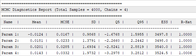
Fig. 4. Example output of summary statistics

Convergence and efficiency diagnostics for the HMC sampler

Now that we have covered the basics of Hamiltonian Monte Carlo, let’s move on to evaluating its practical effectiveness. As a stress test to demonstrate the capabilities of HMC, we will consider a 100-dimensional correlated, heteroscedastic normal distribution. Working with such a complex target distribution (where the variance increases linearly from 1 to 100, and the correlation between neighboring parameters is 0.9) poses a serious challenge for most traditional MCMC algorithms. This example will clearly show the need for preliminary mass matrix tuning to ensure adequate performance in spaces where parameter scales differ greatly.

To do this, we will create a `NormalLogPDF` class that inherits from the abstract `LogPDF` class and implements the log density and analytic gradient required for HMC:

#include <MCMC\HMC.mqh>

// --- HMC INPUT PARAMETERS ---
input int    Inp_Dimension     = 100;   // Dimension of parameter space D
input double Inp_Correlation   = 0.9;   // Correlation coefficient 
input int    Inp_NumChains     = 4;     // Number of chains 
input int    Inp_NumSamples    = 1000;  // Number of stored samples per chain
input int    Inp_ThinSize      = 10;    // Thinning interval
input double Inp_StepSize      = 0.01;  // Initial Leapfrog step size 
input int    Inp_NumLeapfrog   = 50;    // Number of Leapfrog steps
input int    Inp_Burnin        = 1000;  // Warm-up (burn-in) period
input double Inp_TargetAccept  = 0.93;  // Target acceptance probability 
input TUNING Inp_MassTuning    = NONE;  // Mass matrix tuning method
input int    Inp_NumPrint      = 100;   // Frequency of diagnostic output to the log (0 = disabled)

//--- Example LogPDF implementation (correlated multivariate normal distribution)
class NormalLogPDF : public LogPDF {
private:
    ulong size;        // Dimension D
    vector mu;         // Mean 
    matrix sigma;      // Covariance matrix
    matrix inv_sigma;  // Inverse covariance matrix

public:
    NormalLogPDF(ulong dim, double correlation) {
        size = dim;
        mu = vector::Zeros(size);
        sigma = matrix::Zeros(size, size);
        
        // 1. Define a variance scaling vector (from 1.0 to 100.0)
        vector k = vector::Zeros(size);
        for (int i = 0; i <(int) size; i++) {
            double variance_scale = 1.0 + (double)i / (double)(size - 1) * 99.0;
            k[i] = variance_scale;
        }

        // 2. Create a correlated matrix with different variances
        for (int i = 0; i <(int) size; i++) {
            for (int j = 0; j <(int) size; j++) {
                // Covariance Sigma[i, j] = sqrt(k[i] * k[j]) * correlation^|i-j|
                sigma[i, j] = MathSqrt(k[i] * k[j]) * MathPow(correlation, (double)MathAbs(i - j));
            }
        }
        
        // 3. Invert the covariance matrix
        inv_sigma = sigma.Inv(); 
    }
    
    double LogTarget(const vector &z) override {
        vector diff = z - mu;
        return -0.5 * diff @ inv_sigma @ diff;
    }

    vector GradLogTarget(const vector &z) override {
        vector diff = z - mu;
        return -1 * (inv_sigma @ diff);
    }
    
};

First, we will use the EstimateMAP function to find the point of maximum density, which will serve as the optimal starting position.

To comprehensively evaluate the convergence and quality of the resulting sample, we will generate 4 independent chains of 1,000 samples each (after the warm-up period) and calculate key statistics across all chains.

To assess the practical significance of adaptive mass matrix tuning, we will conduct a comparative analysis of two strategies:

• when the mass matrix is not adapted and remains the identity matrix — this is the standard default approach, in which parameter scaling is not taken into account,
• iterative sampling, in which the diagonal elements of the mass matrix are estimated from the sample variances.

Although, in theory, the optimal approach in the Gaussian case would be mass matrix tuning based on the Hessian at the MAP point, in real-world problems involving departures from normality (heavy tails, multimodality, asymmetry), it does not yield satisfactory results. A more reliable and versatile approach is iterative sampling.

Therefore, to demonstrate the capabilities of HMC in realistic scenarios, we will use this approach and compare its results with those of the baseline strategy without adaptation.

//+------------------------------------------------------------------+
//| Script program start function                                    |
//+------------------------------------------------------------------+
void OnStart() {
    int dim =        Inp_Dimension;
    int num_chains = Inp_NumChains;
    Print("--- Start HMC (D=", dim, ", Chains=", num_chains, ") ---");    
    
    // Create an object for the target density
    NormalLogPDF log_pdf(dim, Inp_Correlation);
    
    // 1. Initialize HMC parameters 
    HMC_Params params;
    
    params.num_samples        = Inp_NumSamples;
    params.ThinSize           = Inp_ThinSize;
    params.step_size          = Inp_StepSize;
    params.num_leapfrog       = Inp_NumLeapfrog;
    params.burnin             = Inp_Burnin;
    params.target_accept      = Inp_TargetAccept;
    params.mass_tuning_method = Inp_MassTuning; 
    params.num_print          = Inp_NumPrint;

    // Create an HMC sampler
    HamiltonianSampler mcmc;
      
    // 2. Tune the mass matrix M
    vector initial_point_for_tuning = vector::Ones(dim) * 5.0; // Shifted initial point
    vector mass_vec_out;
    vector endpoint_out(dim); // Final point after mass matrix tuning / warm start

    if (params.mass_tuning_method != NONE)
    {
        Print("--- Estimate MAP Point --- ");
        // Use the MAP result as the starting point for the sampler
        initial_point_for_tuning = mcmc.EstimateMAP(&log_pdf, initial_point_for_tuning); 

        Print(" --- Tune Mass Matrix --- ");  
           if (params.mass_tuning_method == HESSIAN)
        {
             params.mass_vector = mcmc.TuneHessian(&log_pdf, initial_point_for_tuning);        
        } else if (params.mass_tuning_method == ITERATIVE)
        {
            mass_vec_out.Resize(dim);
            endpoint_out.Resize(dim);
            mcmc.TuneIterativeSampling(&log_pdf, params, initial_point_for_tuning, 
                mass_vec_out, endpoint_out);
             
            params.mass_vector = mass_vec_out; 
        }                      
        Print("Mass matrix configuration complete (first 5 and last 5 elements):");       
        int total_size = (int)params.mass_vector.Size();
        int limit_start = (int)MathMin(total_size, 5);       
        // Output the first 5 elements
        for(int i = 0; i < limit_start; i++)
        {
            Print("M[", i, "] = ", params.mass_vector[i]);
        }
        
        if (total_size > 10) // and the last 5
        {
            Print("...");
            int start_index = total_size - 5;                     
            for(int i = start_index; i < total_size; i++) 
            {
                Print("M[", i, "] = ", params.mass_vector[i]);
            }
        }
    }
    // -------------------------------------------------------------    
    // 3. Running HMC for the specified number of chains
    // -------------------------------------------------------------   
    matrix samples_all[]; // Array of all chains
    ArrayResize(samples_all, num_chains);       
    uint start_time = GetTickCount(); 
    for (int chain_idx = 0; chain_idx < num_chains; chain_idx++) 
    {
        Print("\n" + "========================================");
        Print("Start chain #", chain_idx + 1, " from ", num_chains);
        Print("========================================");
        
        vector start_point(dim);      
        if (chain_idx == 0 && params.mass_tuning_method != NONE)
        {
            // For the first chain, we use the final point after tuning.
            start_point = endpoint_out;
            Print("Start point: after adaptation");
        }
        else
        {
            // For the remaining chains, we use a random point to check convergence.
            double rndn[];
            MathRandomNormal(0.0, 5.0, dim, rndn); 
            start_point.Assign(rndn);
            Print("Start point: Random");
        }

        matrix samples = matrix::Zeros(1,1);
        double accept_rate = 0.0;
        vector final_endpoint(dim);        
        mcmc.HMC(start_point, samples, accept_rate, &log_pdf, params, final_endpoint);
        samples_all[chain_idx] = samples;
        Print("--- HMC results for chain #", chain_idx + 1, " ---");
        Print("Acceptance probability: ", DoubleToString(accept_rate * 100, 2), "%");
        // Save samples to a CSV file
        string file_name = StringFormat("HMC/hmc_samples_chain_%d.csv", chain_idx + 1);
        MatrixToCSV(file_name, samples); 
    }  
    uint elapsed_time = GetTickCount() - start_time;
    Print("\nTotal sampling time (", num_chains, " chains): ", DoubleToString(elapsed_time / 1000.0, 3), " seconds");
     
    // 5. Write the sample statistics to the log 
    Diagnostics(samples_all,50, true);
}

Once sampling is complete, we will perform diagnostics across all chains.

Parameter	ESS with M tuning	ESS without M tuning (identity matrix)
param 1	3,370	3,453
param 50	2414	2023
param 80	2915	1552
param 90	2534	1311
param 100	2,669	1715

First, we look at ESS, since it is a key measure of efficiency. The results confirm the importance of adaptation, especially for parameters with high variance. The ESS gain reaches 50–100% when tuning is used. For the parameter with the lowest variance (Param 1), the ESS was 3,370 with adaptation and 3,453 without it — the difference is negligible, since the identity mass matrix is already close to optimal in narrow directions.

R-hat convergence criterion

Parameter	R-hat with M	R-hat without M
All	1 - 1.0025	1 - 1.0020

Both strategies demonstrate excellent convergence (R-hat < 1.01), which means that all four chains have successfully converged to the stationary distribution. However, as ESS shows, convergence does not guarantee efficiency: R-hat indicates convergence, but says nothing about the quality of the samples obtained.

The Monte Carlo standard error (MCSE) is lower when using mass matrix tuning, especially for parameters with a large scale. This means that, for the same number of iterations, tuned HMC provides more accurate estimates of the mean — especially for parameters with high variance.

Parameter	MCSE with M	MCSE without M
param 50	0.1456	0.1536
param 90	0.1859	0.2627
param 100	0.1930	0.2444

The standard deviation (SD) estimates in both cases were virtually identical and very close to the theoretical values:

Parameter	SD with M	SD without M
param 1	0.99	1.00
param 50	7.15	6.91
param 100	9.97	10.12

Minor differences (within 1–3%) are not statistically significant and fall within the range of natural Monte Carlo variation. The SD estimate is almost independent of adaptation; therefore, even with high autocorrelation, if the chains have converged (Rhat < 1.01), the variance will be correct — it will simply converge more slowly.

The key difference lies not in the SD, but in the mean estimates. Without M tuning, there was a noticeable drift in the mean estimates toward negative values (from -0.40 to -0.23), whereas with M tuning, the means remained more symmetric and closer to the true zero (from +0.05 to +0.27). This is further evidence that M adaptation enables a more comprehensive exploration of the state space.

Thus, mass matrix tuning is critical for efficient HMC performance in high-dimensional, heteroscedastic models. HMC is very sensitive to parameter scale, and without mass matrix tuning, “heavy” parameters (those with large variance) move slowly, resulting in high autocorrelation and low ESS.

Although numerical statistical metrics provide objective evidence of successful sampling, it is also useful to visually assess the results of HMC to confirm convergence and examine the shape of the target distribution.

Two main types of plots are used to visualize the results:

• Corner Plot, which displays the marginal univariate distributions of each variable, as well as the pairwise bivariate distributions (i.e., the covariance relationships between each pair of variables):

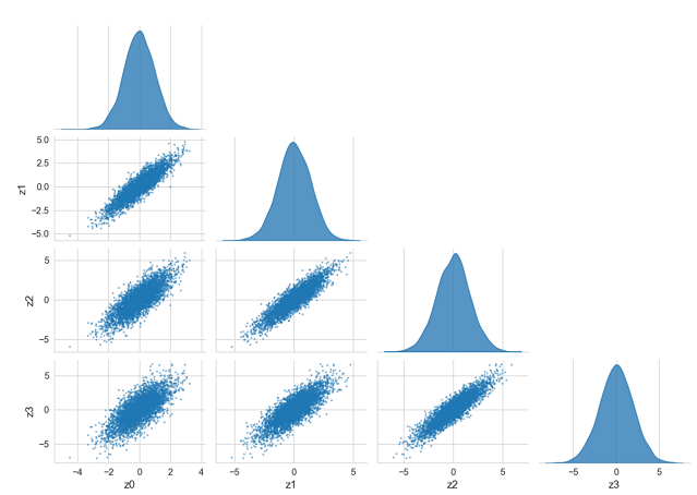
Fig. 5. Corner plot for the first four parameters

• Trace plot, which shows the evolution of parameter values over iterations in each of the four chains. Used to visually check stationarity (the absence of trends), mixing quality, and the absence of autocorrelation:

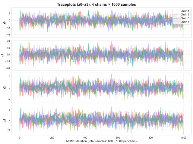
Fig. 6. Trace plot: four chains for the first four variables

Conclusion

This article presented a basic implementation of the Hamiltonian Monte Carlo (HMC) algorithm in the MQL5 language. The effectiveness of the developed gradient sampler was successfully demonstrated using a complex test example — sampling from a 100-dimensional, correlated, and heteroscedastic normal distribution.

The developed functionality is a comprehensive solution that includes the following key components:

• finding a starting point (MAP estimate) using the L-BFGS optimizer,
• checking the correctness of the gradient calculation,
• mass matrix tuning methods,
• comprehensive sample quality diagnostics (Rhat, ESS, MCSE, quantiles),
• real-time monitoring of the sampling process

All of this makes HMC a tool that is ready for practical use in real-world machine learning tasks. It is no coincidence that HMC is called the “gold standard” in Markov chain Monte Carlo. It opens the door to high-dimensional Bayesian modeling, where traditional Markov chain Monte Carlo methods cannot provide sufficient speed and sample quality.

Further development of this method may involve implementing the NUTS (No-U-Turn Sampler) algorithm, which automatically tunes the optimal trajectory length; this would make HMC even more autonomous and reliable by eliminating the need to manually set the number of steps L.

Programs used in the article

#	Name	Type	Description
1	HMC.mqh	Include file	HMC algorithm, mass matrix tuning methods, MAP estimation, sample diagnostics
2	HMC_D100.mq5	Script	Example of sampling with HMC
3	Plot.py	Script	Visualization in Python