MetaTrader 5 Machine Learning Blueprint (Part 19): Bagging Regimes

Table of Contents

1. Introduction
2. The Mechanism AFML Claims
3. Four Regimes Over One Base Learner
4. Metrics: Mechanism First, Efficacy Second
5. The Estimator Confound
6. What the Sequential Draw Buys in Uniqueness
7. Where the Decorrelation Actually Comes From
8. Efficacy and the Permutation Test
9. Out-of-Bag Inflation and Calibration
10. Replication at Higher Event Density (M5 Bars)
11. From Python to MQL5
12. Conclusion
13. Attached Files

Introduction

Part 4 of this series introduced label concurrency, Part 5 implemented the sequential bootstrap, and Part 18 corrected two bugs in the bagging classifier that carries it. Across all three, one link in the argument was assumed rather than measured. AFML §6.2 attributes the failure of bagging on overlapping labels to correlated base learners, and §4.5 prescribes the sequential bootstrap as the fix. The unstated claim is that switching from the standard bootstrap to the sequential one is what decorrelates the trees. This article measures whether it does.

The question matters because the sequential draw is not free. It requires a Numba-compiled sampler. It runs one tree at a time rather than as a vectorized batch. It also complicates downstream folds, which must re-key the sampler to each training subset. If a plain bootstrap with a smaller draw count reaches the same decorrelation, the sequential machinery is a cost without a return. So instead of comparing the sequential bootstrap against a naive baseline and declaring victory, we decompose the change into its two independent parts and measure each one.

The two parts are the draw count and the draw rule. Moving from a standard full bootstrap to a sequential bootstrap at average uniqueness changes both at once: it draws fewer rows, and it draws them by a different rule. To attribute any decorrelation to the right cause, both levers have to move independently. That is what the four-regime design does, and the result is a clean qualification of the AFML mechanism: on this data the draw count does the work, and the sequential draw rule adds almost nothing beyond that.

The Mechanism AFML Claims

The variance of a bagged ensemble of N base learners, each with variance σ² and average pairwise correlation ρ, is the AFML §6.2 expression ρσ² + (1−ρ)σ²/N. As N grows the second term vanishes, but the first does not. It is floored by ρσ². Bagging reduces variance only to the extent that the base learners are decorrelated, and no number of trees rescues an ensemble whose ρ is stuck high.

Overlapping triple-barrier labels push ρ up. An event opened at bar t may not resolve until bar t + 20, so a run of consecutive events shares most of its outcome window. A standard bootstrap draws with replacement from these near-duplicate rows, so two trees see substantially the same information and agree more than independent trees would. Average uniqueness, from AFML §4.4, quantifies the redundancy: it is the mean over each event's lifespan of one divided by the number of concurrent events. On the EURUSD tick bars used here it is 0.435, meaning the effective independent sample is well under half the nominal row count.

AFML §4.5 offers the sequential bootstrap as the remedy. Rather than drawing uniformly, it draws each successive index with a probability that falls as its overlap with the already-drawn set rises, so the sampled set is steered toward low concurrency. The claim under test is specific: that this draw rule, and not merely the reduced draw count that usually accompanies it, is what lowers ρ.

Four Regimes Over One Base Learner

Four ensembles are compared, each 200 trees scored under identical PurgedKFold. Every regime bags the same base learner, so the only thing that varies is the row sampler.

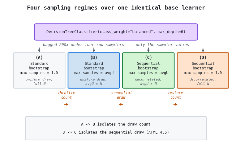
Figure 1. Four-regime illustration of the sampler decomposition

• Regime A: standard bootstrap at max_samples 1.0, the full-count uniform draw that a default bagging classifier performs.
• Regime B: standard bootstrap at max_samples equal to average uniqueness, which throttles the draw count without changing the draw rule.
• Regime C: sequential bootstrap at max_samples equal to average uniqueness, which applies the decorrelating draw rule at the throttled count.
• Regime D: sequential bootstrap at max_samples 1.0, the decorrelating draw rule at the full count.

The comparisons are read off adjacent regimes. A to B isolates the effect of the draw count with the rule held fixed. B to C isolates the effect of the sequential draw rule with the count held fixed, which is the pure test of AFML §4.5. C to D checks whether the sequential rule still helps once the count is no longer throttled. Because a single base learner is bagged throughout, no difference between regimes can be blamed on the estimator.

Metrics: Mechanism First, Efficacy Second

The headline is the mechanism, not the scoreboard. Five quantities are reported per regime. The first two are the mechanism itself: the realized draw uniqueness, measured as the average uniqueness of the rows each tree actually draws relative to the full-sample baseline. The between-tree correlation is measured as the mean pairwise correlation of the trees' out-of-bag probability predictions. The between-tree correlation is the ρ of the §6.2 expression made observable, and it is the quantity the sequential bootstrap is supposed to move.

The remaining three are downstream. Purged-CV out-of-sample AUC is the efficacy readout. We report a permutation test for the main pairwise difference because the companion efficacy study showed that a sub-2% change in event count can shift AUC by roughly 0.10. The gap between out-of-bag accuracy and purged-CV accuracy is a redundancy diagnostic in its own right, because AFML warns that the out-of-bag score is inflated when the samples are redundant. The Brier score reports calibration, which matters because the deployed model feeds bet_size_probability.

The Estimator Confound

The first version of this experiment used a RandomForestClassifier for regimes A and B and the sequential bagging classifier for C and D. That design is broken, and the reason is worth stating because it is easy to miss. A random forest does not only bootstrap rows; it also samples a random subset of features at every split. Feature subsampling is itself a decorrelation mechanism, and a different one from row sampling. With a forest on one side and a bagged tree on the other, any change in between-tree correlation from A to C mixes the row-sampler effect with the presence or absence of feature subsampling, and the two cannot be separated.

The fix is to bag the same DecisionTreeClassifier across all four regimes (class_weight="balanced"). Feature subsampling is disabled everywhere, so the row sampler is the only changing component. This is the single most important design decision in the study. Without it, the clean B-to-C contrast that answers the actual question does not exist.

What the Sequential Draw Buys in Uniqueness

The sequential draw does what it claims at the level of the drawn rows. Panel (a) of the figure below reports the mean uniqueness of each tree's draw, divided by the full-sample baseline.

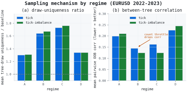
Figure 2. Two-panel illustration of the sampling mechanism by regime

• Panel (a): draw-uniqueness ratio. Throttling the count lifts it from 1.30 at regime A to 1.64 at regime B, and the sequential draw lifts it further to 1.73 at regime C; the full-count sequential regime D falls back to 1.34.
• Panel (b): between-tree correlation, where lower is more decorrelated. The drop is concentrated in the A-to-B step; the B-to-C step is flat or slightly adverse, and regime D is the least decorrelated of all four.

Read panel (a) along the intended path. Regime A draws the full count uniformly and lands at 1.30, above the baseline because a bootstrap of size N contains only about 63% distinct rows. Throttling the count to average uniqueness at regime B lifts the ratio to 1.64. Applying the sequential rule at that same count at regime C lifts it again to 1.73, a further 6% on tick bars and 5% on tick-imbalance bars. The sequential draw genuinely raises the uniqueness of the sampled rows at fixed count, which is exactly its stated job. Regime D confirms the count is the dominant term: at full count the sequential rule cannot avoid the redundant rows and the ratio collapses back to 1.34, barely above regime A.

Where the Decorrelation Actually Comes From

Higher draw uniqueness is supposed to translate into lower between-tree correlation, and this is where the mechanism narrative and the data part company. Panel (b) plots the observable ρ. On tick bars it falls from 0.199 at regime A to 0.145 at regime B, a large drop produced entirely by throttling the count with an ordinary bootstrap. The sequential draw at regime C does not continue the fall. It nudges the correlation back up to 0.163. On tick-imbalance bars the two throttled regimes are indistinguishable, at 0.126 for B and 0.125 for C. In neither representation does the sequential draw rule decorrelate the trees more than the plain count reduction already did.

Regime D sharpens the point. The full-count sequential draw is the least decorrelated of the four, at 0.227 on tick and 0.246 on tick-imbalance bars, worse even than the full-count uniform baseline. A sequential draw at full count still touches nearly every row, and the extra concentration it places on the few high-uniqueness rows appears to make the trees agree more, not less. The lever that moves the §6.2 covariance term is the draw count, not the draw rule. This is the central empirical result of the article, and it holds across both bar representations.

Efficacy and the Permutation Test

None of this reaches the scoreboard. Every regime's out-of-sample AUC sits within a hair of the 0.50 no-skill line, between 0.472 and 0.485 across both representations.

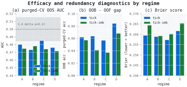
Figure 3. Three-panel illustration of efficacy and redundancy diagnostics

• Panel (a): purged-CV out-of-sample AUC with the shaded no-skill band. Every bar lands inside it, and the best pairwise difference does not clear the permutation test.
• Panel (b): the out-of-bag minus out-of-fold accuracy gap. Regime D carries the largest gap in both representations.
• Panel (c): the Brier score, where regimes B and C are marginally better calibrated than the full-count regimes A and D.

The best-looking regime on tick bars is the throttled sequential arm C, whose AUC of 0.485 sits 0.013 above the baseline A. A Monte Carlo permutation test asks whether that gap means anything. The meta-labels are shuffled, both regimes are re-scored under the same purged cross-validation, and the difference is recorded; the null distribution of the C-minus-A gap has a mean of 0.000 and a standard deviation of 0.008. The observed 0.013 gives a two-sided p-value of 0.125. It does not clear 0.05, and it would clear a Šidák-corrected threshold for the regime grid by an even wider margin. On efficacy, the four regimes are indistinguishable.

This is precisely the "Good Luck" problem that Timothy Masters warns against in Testing and Tuning Market Trading Systems: a backtest or cross-validated result that appears profitable (or, here, slightly better conditioned) can simply be the lucky tail of a null distribution centered at zero. The permutation test provides the statistical safeguard that Masters demands—an explicit counterfactual that asks whether the observed edge would survive if the labels were random. Here, it does not. Echoing the companion finding that better statistical conditioning did not buy strategy efficacy, the p-value confirms that the modest edge of Regime C is indistinguishable from noise.

Out-of-Bag Inflation and Calibration

The out-of-bag score is a tempting shortcut for model selection because it comes free with the fit. Panel (b) shows why it is a trap here. The gap between out-of-bag accuracy and honest purged-CV accuracy is largest for regime D, at 0.084 on tick bars and 0.068 on tick-imbalance bars, precisely the full-count sequential arm that a practitioner following the book most closely might reach for. A model chosen on its out-of-bag score would rank D favorably, while its purged-CV AUC is among the worst and its Brier score is the worst of the four. The out-of-bag estimate is inflated exactly where the draws are most redundant, and the full-count sequential draw is redundant by construction. The practical takeaway is absolute: never use Out-of-Bag scores for model selection when dealing with overlapping financial labels. It is a trap that leads directly to allocating capital to overfit models. 

The calibration panel closes the loop for deployment. The throttled regimes B and C carry the lowest Brier scores, 0.257 to 0.259, while the full-count regimes A and D are worse, up to 0.265. A model that feeds a probability into position sizing should be selected on calibration as much as on AUC, and by that criterion the count-throttled regimes win the modest margin that exists. The practical recommendation that falls out of the whole grid is unglamorous: set max_samples to average uniqueness with an ordinary bootstrap, and treat the sequential draw as a second-order refinement rather than the load-bearing correction the book presents it as.

Replication at Higher Event Density (M5 Bars)

The tick and tick-imbalance bars used above aggregate to roughly one bar an hour, and over two years of EURUSD that yields only 1,269 to 1,289 meta-labeled events. A method whose entire premise is exploiting high-frequency data has no business being validated on an hourly-equivalent sample, and a thin event count is also the more mundane reason the permutation test above could not fully rule out chance. This section repeats the identical four-regime design, unchanged in every respect except the bars, on M5 time bars. M5 yields 11,833 events, roughly nine times the count above, at an average uniqueness of 0.462, in line with the tick-bar value of 0.435.

The M5 replication ran at 60 trees and 4-fold PurgedKFold rather than the primary grid's 200 trees and 5 folds, a lighter setting made necessary by the added cost of the sequential arms at ten times the row count. A preliminary sweep on the tick-bar grid, from 30 to 200 trees, reproduced the same regime ordering throughout, so tree count is not expected to be the deciding factor here. A full 200-tree confirmation at M5 is still the appropriate step before this replication is treated as final. Readers with sufficient compute are encouraged to run the attached notebook at 200 trees; the provided M5 results at 60 trees are offered as a directional replication, not a final word.

Regime	tick corr	tick-imb corr	M5 corr

The ordering that anchors this article's central claim survives entirely intact: the A-to-B step carries the decorrelation, the B-to-C step gives it back a little, and regime D remains the worst of the four. The absolute correlations are lower across the board at M5, and the gap between the best regime (B) and the worst (D) narrows somewhat in relative terms, but the ranking A > D, C ≈ B (with B the marginal best) does not change at nine times the event count. That is the strongest evidence in the article that the effect is real and not an artifact of a thin H1-equivalent sample.

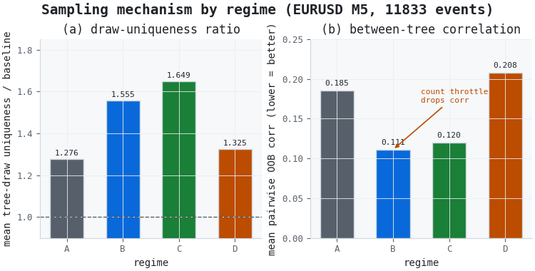
Figure 4. Two-panel illustration of the sampling mechanism at M5

• Panel (a): draw-uniqueness ratio at M5. Regime A sits at 1.28, B at 1.56, C at 1.65, D at 1.32, the same shape as the primary grid.
• Panel (b): between-tree correlation at M5. B is the lowest at 0.111, C a close second at 0.120, and D the highest at 0.208.

The efficacy picture changes in one genuinely new way. At M5 every regime's out-of-sample AUC sits above the 0.50 no-skill line, between 0.511 and 0.520, where the primary grid sat entirely below it. The finer cadence buys a sliver of measurable signal that the coarse bars could not detect. What it does not buy is separation between regimes. The best pairwise delta is now B-minus-A at 0.0047, and a permutation test with a null standard deviation of 0.0036 gives a two-sided p-value of 0.216, weaker evidence for a real gap than the tick-bar result even though the null itself is tighter. More events sharpened the estimate and, in sharpening it, shrank the apparent edge. On efficacy the four regimes remain indistinguishable at an event count that would have had a fair chance of separating them if a true difference existed.

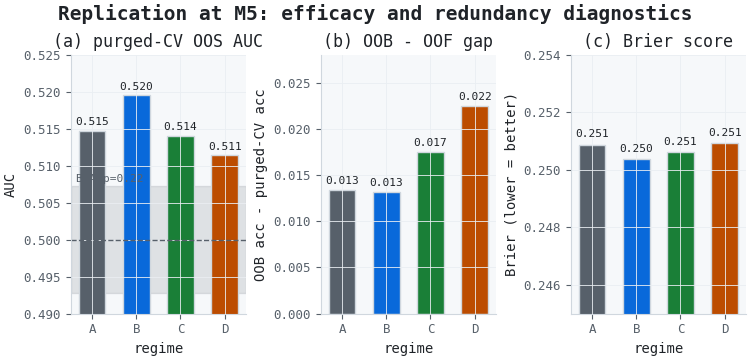
Figure 5. Three-panel illustration of efficacy and redundancy diagnostics at M5

• Panel (a): purged-CV OOS AUC at M5, all four regimes above the no-skill line, with the best pairwise delta annotated.
• Panel (b): the OOB-OOF gap at M5, compressed to 0.013-0.022 from the primary grid's 0.037-0.084, but preserving the same ordering with D worst.
• Panel (c): Brier score at M5, tightly clustered at 0.250-0.251, with B the marginal best.

The out-of-bag inflation diagnostic also holds up, and it sharpens the deployment answer rather than complicating it. Regime D still carries the largest OOB-OOF gap, 0.022 against 0.013 for A and B, the same pattern as the primary grid at roughly a quarter of the absolute magnitude; the larger event count gives the purged-CV estimate itself less room to disagree with the OOB score, but the direction of the disagreement is unchanged. Calibration resolves the ambiguity the primary grid left open. There, B and C were close enough on Brier score that either was a defensible deployment choice. At M5, B is unambiguously the best on both AUC and Brier, while C is no longer distinguishable from A. The sequential draw's one redeeming case at the primary grid, marginal calibration parity with B, does not survive the higher-density replication.

From Python to MQL5

The offline verdict, confirmed at nine times the event count, is that the count-throttled standard bootstrap, regime B, decorrelates best and calibrates best, and that the sequential draw rule adds nothing detectable on efficacy at either bar cadence.

Part 20 will carry this hand-off into the MetaTrader 5 Strategy Tester. Specifically, I will export the Regime B (throttled standard bootstrap) and Regime A (full-count baseline) models to ONNX, wrap them in the meta-labeling Expert Advisor introduced in Part 17, and run both systems on an untouched hold-out year of tick data. The test will measure whether the offline decorrelation benefit translates into higher net profit, lower maximum drawdown, and superior pathwise Sharpe after accounting for the transaction costs modeled in Part 14. The Strategy Tester will also run regimes C and D, so the honest question can be answered directly: does the regime that decorrelated best offline also produce the best tester equity, or does the difference wash out as it did in cross-validation. The key question is whether the statistical conditioning that survives the M5 replication also survives contact with live-mimicking tick-by-tick execution.

Choosing B over C or D is itself worth stating plainly, since it runs against the book's preferred arm. AFML's sequential bootstrap is the tool that C and D carry, and neither the primary grid nor the M5 replication supports paying for it: no efficacy edge, no calibration edge, and a real cost in inference-time complexity from the Numba-compiled sampler. The model that reaches the tester is the one an ordinary bootstrap at a throttled count produces. The bar family the tester trains and runs on should match the M5 replication rather than the coarser primary grid, since M5 is both the higher-power evidence base and the cadence a live ML pipeline is meant to exploit.

That hand-off mirrors the discipline of the companion series. An offline diagnostic is a hypothesis about live behavior, not a substitute for it, and the tester is where the hypothesis is checked against out-of-sample bars the model never touched during selection.

Conclusion

Bagging on overlapping labels does need a correction, and AFML §6.2 diagnoses the problem correctly: redundant draws leave the trees correlated and floor the ensemble variance. However, the correction that matters on a single, highly liquid FX pair like 2022-2023 EURUSD is simply throttling the draw count to average uniqueness. It is entirely possible that across a broad cross-sectional equity universe with different concurrency and momentum dynamics, the sequential draw rule shows its teeth. But here, an ordinary bootstrap at that reduced count captures the entire decorrelation benefit; the sequential draw rule, at the same count, adds nothing measurable to the between-tree correlation and nothing to the out-of-sample AUC. The full-count sequential arm is worse on every axis that matters, including the out-of-bag inflation a careless selection would reward.

This is a qualification of the book, not a contradiction of it. The sequential bootstrap does raise the uniqueness of the sampled rows, exactly as §4.5 says. What the data does not support is the further step that the sequential draw rule is the operative lever for decorrelating the ensemble on this specific instrument. Here, the count is the lever. While the exact dominant mechanism may shift depending on the asset class, the methodological lesson generalizes perfectly: when a prescribed method bundles two changes, decompose it and measure each part before attributing the benefit. The emphasized component is not always the one driving the result. Part 20 carries the four trained models into the Strategy Tester to see whether any of this survives contact with a hold-out year.

Attached Files

The afml/ folder is a minimal excerpt of the Blueprint Quant afml package: only the subpackages this notebook imports, with empty package markers in place of the full package's loader. It requires numba, scipy, statsmodels, and TA-Lib alongside numpy, pandas, and scikit-learn.

	File	Location	Description
1.	Blueprint_Part19_Bagging_Regimes.ipynb	Notebooks\	Reproducible notebook. Builds the labeled dataset from cached tick, tick-imbalance, and M5 bars, runs the four-regime comparison at each cadence, computes the five metrics per regime, and reproduces the permutation tests and every figure.
2.	tick.parquet, tick_imb.parquet, m5.parquet	bars_cache\	Pre-built OHLCV bars the notebook reads directly, so reproducing the article does not require reprocessing the underlying 2022-2023 EURUSD tick history. 12,325 tick bars, 13,220 tick-imbalance bars, and 147,860 M5 bars.
3.	afml/ensemble/, sampling/	afml\	SequentiallyBootstrappedBaggingClassifier and the sequential bootstrap, average uniqueness, and concurrency routines that define the regimes.
4.	afml/strategies/, labeling/	afml\	The primary strategy and the triple-barrier labeling that produce the events and the t1 sets from which average uniqueness is computed.
5.	afml/cross_validation/, data_structures/, filters/, util/, sample_weights/	afml\	PurgedKFold, the bar builders, the CUSUM filter, the volatility target, and sample-weight helpers.