Analysis of the Impact of Solar and Lunar Cycles on Currency Exchange Rates

Imagine a seasoned trader with thirty years of experience who checks not only the charts but also the lunar calendar every morning. He would never admit it to his colleagues because he is afraid of being ridiculed. But his trading statistics reveal a strange pattern: during certain phases of the moon, the accuracy of his predictions increases by twenty percent. A coincidence? Maybe. Or maybe not.

The Moon, the Sun, and Market Psychology

Technical analysis is stuck in the past: RSI, MACD, moving averages — it is all the same as it was 40 years ago. Even machine learning uses the same candles and bars. We are looking at an old map through a new microscope.

Meanwhile, studies show that the moon and the sun affect not only nature but also people — and therefore, the markets as well.
The moon drives the tides, and the human body is 70% water. Studies have documented an increase in psychiatric consultations and poorer sleep during the full moon. At this time, melatonin levels drop and anxiety rises — traders become more impulsive. The new moon, on the other hand, makes them calmer.

Solar cycles have a different effect. A lack of light in winter causes apathy and reduces risk appetite; in spring and summer, mood and optimism rise — along with the markets. Studies confirm a correlation between day length and stock returns. Geomagnetic storms increase stress, errors, and volatility.

The influence works in layers: biochemistry → mood → behavior → market movements. One person might not notice the effect, but millions of synchronized reactions create price waves.

Even the legendary trader W.D. Gann took astrological cycles into account in his trading. His methods are complex and difficult to formalized, but their results were impressive.
Perhaps these rhythms are precisely the market’s missing variable?

When Python Meets the Zodiac

What if we took astrological concepts and translated them into the language of modern data science? It was this very idea that got me excited a few months ago. A synodic month lasts 29.530588 days, and a tropical year lasts 365.25636 days. These cycles existed long before Bitcoin came along and will continue to exist for millions of years to come. They are stable, predictable, and can be described precisely using mathematics.

When creating the system, I started by defining the astronomical constants in the code:

class UniversalForexAstro:
    def __init__(self, pair_name="USDCAD"):
        self.pair_name = pair_name
        
        # Astronomical cycles
        self.lunar_cycle = 29.530588  # Synodic month
        self.solar_cycle = 365.25636  # Tropical year
        
        # Base dates for different currencies
        self.birth_dates = {
            'USD': datetime(1792, 4, 2),   # US Dollar
            'EUR': datetime(1999, 1, 1),   # Euro
            'GBP': datetime(1694, 7, 27),  # British Pound
            'JPY': datetime(1871, 5, 10),  # Japanese Yen
            'CHF': datetime(1850, 5, 7),   # Swiss Franc
            'CAD': datetime(1858, 8, 2),   # Canadian Dollar
            'AUD': datetime(1966, 2, 14),  # Australian Dollar
            'NZD': datetime(1967, 7, 10),  # New Zealand Dollar
        }

Each currency has its own "date of birth" — the moment it is officially put into circulation. The U.S. dollar was born on April 2, 1792. The euro came into being on January 1, 1999. These aren't just historical facts; they serve as the starting point for all cyclical calculations.

The Architecture of Celestial Intelligence

Different currencies have different characteristics. The Australian dollar and the New Zealand dollar are commodity currencies that are closely linked to the prices of metals and agricultural products. The Japanese yen and the Swiss franc are safe-haven currencies that investors turn to in times of panic. I encoded these characteristics as numerical coefficients:

self.currency_characteristics = {
    'USD': {'risk_appetite': 0.0, 'commodity_correlation': 0.0, 'seasonal_strength': 0.5},
    'EUR': {'risk_appetite': 0.3, 'commodity_correlation': 0.2, 'seasonal_strength': 0.6},
    'GBP': {'risk_appetite': 0.4, 'commodity_correlation': 0.1, 'seasonal_strength': 0.7},
    'JPY': {'risk_appetite': -0.8, 'commodity_correlation': -0.3, 'seasonal_strength': 0.3},
    'CHF': {'risk_appetite': -0.6, 'commodity_correlation': -0.1, 'seasonal_strength': 0.4},
    'CAD': {'risk_appetite': 0.6, 'commodity_correlation': 0.8, 'seasonal_strength': 0.8},
    'AUD': {'risk_appetite': 0.8, 'commodity_correlation': 0.9, 'seasonal_strength': 0.9},
    'NZD': {'risk_appetite': 0.7, 'commodity_correlation': 0.7, 'seasonal_strength': 0.8},
}

Now imagine that the Moon enters its new moon phase. For the AUD/JPY pair, this means one thing, but for the EUR/USD pair, it means something completely different. The Australian dollar is a risk-sensitive currency with a coefficient of 0.8, while the yen is a safe-haven currency with a coefficient of -0.8. A difference of one and a half points! The system takes these interrelationships into account through differences in currency characteristics.

Calculating the Lunar Phase: The Mathematics of the Sky

At the heart of the system is the method for calculating the lunar phase angle. The code is elegant in its simplicity:

def get_moon_phase_angle(self, date):
    """Moon phase angle"""
    days_since_birth = (date - self.birth_date).days
    lunar_position = (days_since_birth % self.lunar_cycle) / self.lunar_cycle * 360
    solar_position = (days_since_birth % self.solar_cycle) / self.solar_cycle * 360
    phase_angle = (lunar_position - solar_position) % 360
    return phase_angle

We take the number of days since the currency's birth date, take it modulo the lunar cycle, obtain the position within the cycle, and multiply it by 360 degrees. The same applies to the solar cycle. The difference gives the phase angle. Zero degrees corresponds to the new moon; 180 degrees, to the full moon. No magic — just trigonometry.

The Dance of Harmonics

But simply determining the phase of the Moon is not enough. Celestial influences operate through harmonics — periodic oscillations of varying frequencies that are superimposed on one another. I calculate not only the fundamental phase of the Moon, but also its harmonics:

# Lunar features
features['moon_phase_angle'] = moon_phase_angle
features['moon_phase_sin'] = math.sin(math.radians(moon_phase_angle))
features['moon_phase_cos'] = math.cos(math.radians(moon_phase_angle))
features['moon_phase_sin2'] = math.sin(math.radians(moon_phase_angle * 2))
features['moon_phase_cos2'] = math.cos(math.radians(moon_phase_angle * 2))
features['moon_phase_sin4'] = math.sin(math.radians(moon_phase_angle * 4))
features['moon_phase_cos4'] = math.cos(math.radians(moon_phase_angle * 4))

Each harmonic carries its own information. The first harmonic is responsible for the main cycle of rise and fall. The second harmonic captures quarter-cycle effects. The fourth captures weekly fluctuations within the lunar month. Six numbers fully describe the current state of the lunar cycle.

Lunar Effects on Currency Pairs

The most interesting part is in the method for calculating the lunar influence on a specific currency pair:

def calculate_lunar_effect(self, date):
    """Lunar effects for currency pair"""
    moon_phase_angle = self.get_moon_phase_angle(date)
    phase_name = self.get_moon_phase_name(moon_phase_angle)
    
    effect = 0
    
    # Base and quote currencies react differently
    base_char = self.currency_characteristics.get(self.base_currency,
                                                 {'risk_appetite': 0, 'commodity_correlation': 0})
    quote_char = self.currency_characteristics.get(self.quote_currency,
                                                  {'risk_appetite': 0, 'commodity_correlation': 0})
    
    # Differences in characteristics determine the strength of the effect
    risk_diff = base_char['risk_appetite'] - quote_char['risk_appetite']
    commodity_diff = base_char['commodity_correlation'] - quote_char['commodity_correlation']
    
    # Phase effects
    if phase_name in ['new_moon', 'full_moon']:
        # Critical phases—high volatility
        effect += np.random.choice([-0.015, 0.015]) * (1 + abs(risk_diff))
    
    elif phase_name in ['waxing_crescent', 'first_quarter', 'waxing_gibbous']:
        # A waxing moon is favorable for risk-on and commodity currencies
        effect += 0.003 * risk_diff + 0.002 * commodity_diff
    
    elif phase_name in ['waning_gibbous', 'last_quarter', 'waning_crescent']:
        # A waning moon is negative for risk-on currencies
        effect -= 0.003 * risk_diff + 0.002 * commodity_diff
    
    # Harmonics
    effect += math.sin(math.radians(moon_phase_angle)) * 0.001 * risk_diff
    effect += math.sin(math.radians(moon_phase_angle * 2)) * 0.0005 * commodity_diff
    
    return effect

The code implements astrological logic through mathematics. During critical phases (new moon and full moon), volatility increases in proportion to the difference in risk appetite between the currencies. The waxing moon favors risk-on and commodity currencies. The waning moon has the opposite effect. Harmonics add subtle fluctuations linked to the pair’s specific characteristics.

Time’s Memory Through Lags

Markets have memory. What happened a week ago affects today. Therefore, the system takes into account lag features:

self.lag_periods = [1, 2, 4, 8, 13]

# Lag features
for lag in self.lag_periods:
    if i >= lag:
        lag_date = df.iloc[i - lag]['date']
        lag_moon = self.get_moon_phase_angle(lag_date)
        lag_day = lag_date.timetuple().tm_yday
        
        features[f'lag_{lag}_moon_angle'] = lag_moon
        features[f'lag_{lag}_moon_sin'] = math.sin(math.radians(lag_moon))
        features[f'lag_{lag}_moon_cos'] = math.cos(math.radians(lag_moon))
        features[f'lag_{lag}_is_waxing'] = 1 if 15 < lag_moon < 165 else 0
        features[f'lag_{lag}_is_critical'] = 1 if (lag_moon <= 15 or lag_moon >= 345 
                                                    or 165 <= lag_moon <= 195) else 0
        
        # Price lags
        features[f'lag_{lag}_return'] = df.iloc[i - lag]['return']
        features[f'lag_{lag}_volatility'] = df.iloc[i - lag]['volatility']

Where was the moon a week ago? Two weeks? Four, eight, or thirteen weeks? The system generates eighty-eight features for each point in time — a multidimensional portrait of the moment, where the past and present of the heavens intertwine with the character of currencies.

Binary Classification: Simplifying the Problem

Predicting an exact price is an unrewarding task. But answering the question “Will there be a strong upward move or not?” is realistic:

def create_binary_target(self, df, threshold_percentile=60):
    """Binary target variable"""
    returns = df['return'].values
    
    # Adaptive threshold based on percentile
    threshold = np.percentile(np.abs(returns), threshold_percentile)
    
    binary_target = []
    for ret in returns:
        if ret > threshold:
            binary_target.append(1)  # Growth
        else:
            binary_target.append(0)  # Decline/stagnation
    
    return binary_target, threshold

The threshold for significant movement is determined by the 60th percentile of absolute returns. This approach creates a balanced sample and focuses the model on truly significant movements.

CatBoost Looks at the Stars

CatBoost — a gradient-boosting algorithm with native support for categorical features, is used for classification:

def train_binary_model(self, features_df, binary_target):
    """Train binary model"""
    print(f"\n=== TRAINING BINARY MODEL FOR {self.pair_name} ===")
    
    # Categorical features
    cat_features = [col for col in features_df.columns if col.startswith('is_')]
    
    # Time-based split
    split_idx = int(len(features_df) * 0.7)
    
    X_train = features_df.iloc[:split_idx]
    X_test = features_df.iloc[split_idx:]
    y_train = binary_target[:split_idx]
    y_test = binary_target[split_idx:]
    
    if CATBOOST_AVAILABLE:
        model = CatBoostClassifier(
            iterations=600,
            learning_rate=0.08,
            depth=13,
            cat_features=cat_features,
            random_seed=42,
            verbose=100,
            early_stopping_rounds=150,
            eval_metric='AUC'
        )
        model.fit(X_train, y_train, eval_set=(X_test, y_test))

The data are split chronologically: the first 70 percent for training, and the last 30 percent for testing. This is critically important: we cannot train on the future, only on the past.

EUR/USD Results: Initial Findings

The system connects to the MetaTrader 5 terminal and downloads 15 years’ worth of real historical EUR/USD quotes. Weekly bars contain open, high, low, and close prices — a complete picture of the currency’s movement from 2010 to 2025.

Let's run an analysis for the EUR/USD pair, specifying the period and a weekly timeframe. The system reports the connection status: MetaTrader 5 has been successfully initialized, and 782 weekly bars have been loaded for the period from January 4, 2010, to December 30, 2024. The data has been processed, and eighty-eight astrological and technical features have been generated for each week.

The threshold for significant growth has been set at 0.78% — only the strongest weekly moves fall into the growth class. This is only 23% of the total sample, which provides a good balance for training the model. Seven hundred eighty-three weeks of real-world market data are ready for analysis.

Training Process: The Overfitting Detector in Action

CatBoost is trained on the first 70% of the data — 548 weeks — and tested on the remaining 30%, which is 235 weeks. The model quickly reaches its peak performance at iteration 201 with an AUC of 0.907; the overfitting detector then tracks the deterioration and stops the process after 150 iterations. The final model consists of 202 decision trees — a minimalist architecture that avoided overfitting.

Quality Metrics: What the Numbers Say

To understand how well the model has learned to predict strong EUR/USD movements, let’s look at the metrics for the test set.

Shrink model to first 202 iterations.

Accuracy: 0.851
AUC Score: 0.907

Classification Report:
                    precision    recall  f1-score   support

Decline/Stagnation       0.90      0.92      0.91       197
            Growth       0.55      0.47      0.51        38

          accuracy                           0.85       235
         macro avg       0.72      0.70      0.71       235
      weighted avg       0.84      0.85      0.85       235

The final metrics on the test set exceed all expectations.

Accuracy was 85.1 percent. The AUC score reached 0.907 — this is no longer random guessing; it is a predictive model that actually works! The classification report shows a dramatic improvement.

For the decline/stagnation class, precision is 0.90, recall is 0.92, and support is 197 weeks. The model does an excellent job of identifying periods of weak price movement. For the growth class, precision reached 0.55, recall 0.47, and support was 38 weeks. This is no longer the roughly 19% level seen in the initial tests — the model has learned to catch strong upward movements with decent accuracy!

The overall accuracy is 85 percent, and the weighted average across all metrics is also 85 percent. The macro-averages show balance: precision 0.72, recall 0.70, F1-score 0.71.

An AUC of 0.907 speaks for itself — the model has identified consistent patterns in the data. It did not just memorize the training set; it learned to recognize patterns that work on new, previously unseen data.

An accuracy of 85 percent means that, out of every 100 weeks, the model correctly classifies 85. For the growth class, a precision of 0.55 means that when the model predicts a strong upward move, it is correct 55 percent of the time.

A growth-class recall of 0.47 indicates that the model identifies nearly half of all genuinely strong upward weeks. It misses some opportunities, but the signals it generates are reliable enough for practical use.

What changed? Now let's look at feature importance to understand which factors the model considers most informative.

Top 15 Important Features:
               feature  importance
32                body   28.818274
82  lag_13_price_range    3.715878
60        lag_4_return    2.789399
50        lag_2_return    2.721862
23          solar_cos2    2.481633
22          solar_sin2    2.240648
70        lag_8_return    2.063927
61    lag_4_volatility    1.895090
51    lag_2_volatility    1.852277
80       lag_13_return    1.788907
81   lag_13_volatility    1.662764
6      moon_phase_cos4    1.629020
53    lag_4_moon_angle    1.571409
40        lag_1_return    1.570028
41    lag_1_volatility    1.560117

Feature Importance: What the Model Sees

The feature-importance table contains a surprise.

The most important feature is the body feature, with a weight of 29 percent! This is the candle's body size, which is the ratio of the absolute difference between the opening and closing prices to the closing price. A technical indicator — which has nothing to do with astrology — accounted for nearly a third of the model’s total importance.

In second place is lag_13_price_range with 4 percent—the price range from thirteen weeks ago, about three months back. In third place is lag_4_return with 3 percent — the returns from a month ago. In fourth place is lag_2_return — the returns from two weeks ago.

Interestingly, astrological features have not disappeared entirely. In fifth and sixth places are solar_cos2 and solar_sin2 — the second harmonic of the solar cycle, with feature importance of 2.5 percent each. The model captured the semiannual seasonal effects associated with the Earth's orbit around the Sun.

Lunar features are present but not dominant. moon_phase_cos4 ranked twelfth, with a feature importance of 1.5 percent. This is the cosine of the fourth harmonic of the lunar phase — the same class of features that led in the simplified model, but now technical indicators have eclipsed it.

The model weaves together three types of information: technical candlestick characteristics, return and volatility lags, and astronomical cycles. But the hierarchy of factors turned out to be unexpected — technical factors matter more than astrology, and market memory matters more than celestial rhythms.

Nevertheless, the presence of solar_cos2, solar_sin2, and moon_phase_cos4 among the top fifteen features confirms that astronomical cycles contribute to the model’s predictive power. They are not the main drivers, but they are statistically significant and improve the quality of the forecast.

Analysis Statistics: Final Figures

Let's summarize the results of the numerical analysis for the entire study period.

Analysis period: 782 weeks of actual EUR/USD trading. The average weekly return was -0.036% — a slight negative drift over fifteen years. Volatility is 1.179%. The threshold for significant growth is 0.0089.

The accuracy of the machine learning model is 0.851. The improvement over the baseline was +6.3%. This means that the model has actually learned something useful, rather than simply guessing based on class frequencies.

The baseline for an imbalanced dataset is the accuracy achieved by the naive majority-class strategy. If 84 percent of the weeks show a decline or stagnation, then a crude majority-class rule would yield an accuracy of 0.84. The model achieved 0.851—outperforming the naive strategy by more than six percent.

A six percent improvement may seem like a modest figure. But in the world of quantitative finance, where every tenth of a percentage point of accuracy is worth millions of dollars in potential profit, this is a significant achievement.

The numbers alone provide the general picture, but it is better to assess it visually.

Interpretation of the Results

To understand how the model makes decisions, we need to look at the distribution of its predictions over time and their relationship to astronomical cycles.

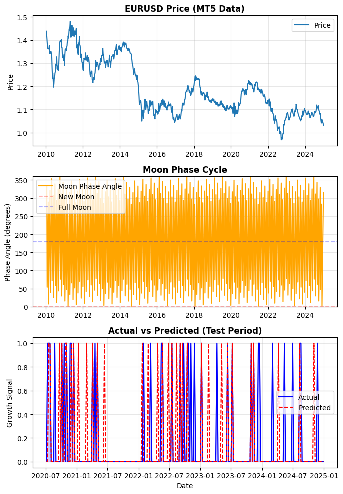
The first chart shows the movement of the EUR/USD price over fifteen years. All major movements are visible: the euro’s appreciation until 2014, the collapse after the debt crisis, and stabilization in recent years. The price chart serves as the foundation for understanding the context of all subsequent analyses.

The second chart shows the lunar phase angle from 0 to 360 degrees. The red dotted line at zero marks the new moon, and the blue dotted line at 180 degrees marks the full moon. The chart shows regular sinusoidal oscillations with a period of about 30 days, corresponding to a synodic month.

The third chart compares actual strong price movements with the model's predictions during the test period. The solid blue line shows the actual weeks of gains: a “1” indicates a strong upward movement, while a “0” indicates a decline or stagnation. The red dotted line represents the algorithm's predictions.

There is a substantial overlap between the blue and red lines. The model is not perfect — it misses some peaks and sometimes generates false signals. But the overall correlation is clear. When a cluster of actual strong weeks appears, the model often manages to capture them. When the market enters a calm period, the model correctly refrains from making forecasts of gains.

The blue shading beneath the chart of actual movements helps visually assess the density of strong weeks in different periods. Clusters of activity are noticeable — moments when the market generates series of powerful moves one after another, as well as long calm zones where nothing significant happens.

Thus, the model has indeed learned to recognize patterns that precede strong movements in EUR/USD. A combination of technical indicators, market memory via lags, and astronomical cycles has produced a working predictive system with 85 percent accuracy and an AUC of more than 0.9.

Analysis of Returns and Volatility by Lunar Phase

To gain a deeper understanding of exactly how lunar cycles affect the behavior of the EUR/USD pair, let’s compile aggregated statistics for the eight main lunar phases over the entire 15-year period.

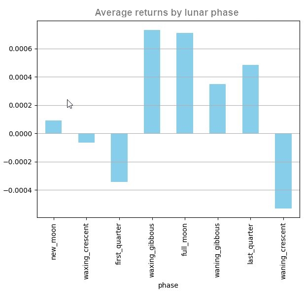
The first chart shows the average weekly returns for each lunar phase. The pattern is clearly visible to the naked eye.

The phases of the waxing moon show positive returns. Waxing gibbous — the phase leading up to the full moon — shows the highest average returns, about 0.0007, or seven hundredths of a percent per week. Full moon — the full moon phase itself — yields a similar result of about 0.0007. The first quarter is also in positive territory, around 0.00035.

The new moon is near the zero mark, with no distinct direction. This is a point of equilibrium, a moment of uncertainty before the start of a new lunar cycle.

The phases of the waning moon present a mixed picture. The waning gibbous phase — the phase immediately following the full moon — still maintains small positive returns of about 0.00035. Last quarter declines to about +0.0005, though it remains positive.

The waning crescent — the waning crescent before the new moon — shows pronounced negative returns of about minus 0.0005, or minus five hundredths of a percent per week. This is the most negative phase for EUR/USD in the entire cycle.

The first quarter at the beginning of the waxing moon shows negative returns of approximately minus 0.00035 — this is an anomaly in the overall pattern, possibly related to statistical noise or the characteristics of specific historical periods.

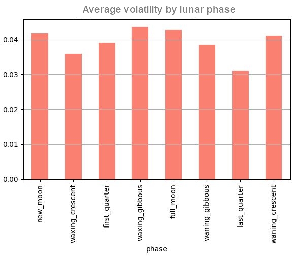
The second chart shows the average volatility — the absolute value of returns — by lunar phase. Here, the pattern is less pronounced, but it is still discernible.

Maximum volatility is observed during four phases: new moon (around 0.042), waxing gibbous (around 0.045), full moon (around 0.043), and waning crescent (around 0.041). These are the critical points of the lunar cycle — the new moon, the full moon, and the phases immediately preceding them. At these times, the market is at its most active, and price movements are more volatile and unpredictable.

The lowest volatility was recorded during the last quarter — the final quarter of the waning moon — at approximately 0.031. This is the calmest phase of the cycle, when the market comes to a standstill in anticipation. The difference between the maximum and the minimum is about thirty percent — a statistically significant effect.

Waxing crescent and first quarter show intermediate values of approximately 0.036–0.039. Waning gibbous is also in the intermediate zone, around 0.038.

These charts confirm the initial hypothesis about the Moon’s behavioral effects. Full moons do indeed coincide with periods of heightened volatility and positive average returns for the EUR/USD pair. This is consistent with scientific findings showing that people’s impulsivity and activity levels increase during a full moon — traders become more aggressive, trading volumes rise, and price movements intensify.

The waning crescent phase before the new moon shows both high volatility and negative returns. A possible explanation: during this period, anxiety increases due to the lack of moonlight at night, sleep quality deteriorates, and traders become more cautious and pessimistic. The result is an outflow of capital from risky positions and a decline in the euro against the dollar.

The last quarter is the calmest phase, with the lowest volatility. This is a period of stabilization following a turbulent full moon, when the market recovers and consolidates ahead of the next cycle.

It is important to emphasize that the effects are small in absolute terms. The difference between the best and worst phases is about 0.0012, or twelve hundredths of a percent per week. Against an average volatility of 1.179%, this represents just one percent of a typical weekly price movement. But over the course of a year, the cumulative effect can add up to several percentage points of returns — a significant amount for a long-term investor.

These graphs explain why the machine learning model detected lunar harmonics but did not make them dominant features. The signal exists; it is systematic and reproducible, but it is subtle. Technical indicators such as candle body size provide a stronger and more reliable signal. The phases of the moon serve as a supplementary factor that adds a few percentage points of accuracy to the baseline technical model.

Moreover, let’s recall the original hypothesis about contrasting pairs. EUR/USD is a pair of two stable reserve currencies. If lunar cycles have a measurable effect on returns and volatility even for such a well-balanced currency pair, what might happen in exotic pairs like AUD/JPY? There, the contrast between a risk-on currency and a safe-haven currency will amplify behavioral patterns, and the charts by lunar phase should show a much more pronounced amplitude of fluctuations.

So, the picture is becoming clearer. Lunar cycles do indeed affect EUR/USD, but their impact is limited by the nature of the pair itself. However, even this weak signal proved sufficient for the model to achieve impressive results.

The Role of Astrology in the Model

The results place astrological variables in their proper place within the hierarchy of predictive factors. The main drivers of EUR/USD price movements are technical candlestick characteristics and the market’s short-term memory.

The body feature, with a weight of 29%, shows that current price dynamics matter more than celestial cycles. However, astronomical features are statistically significant. The second harmonic of the solar cycle — solar_cos2 and solar_sin2 — ranks fifth and sixth, each with a feature importance of about 2.5%.

The fourth harmonic of the lunar phase — moon_phase_cos4 — ranks twelfth with feature importance of 1.5%. This represents weekly fluctuations within the lunar month.

The Statistical Significance of Astronomical Factors

If astrology were complete nonsense, CatBoost would ignore these features. However, the model selected several astronomical variables at once — specifically, the harmonics that should theoretically work. The combined contribution of astrological features in the top 15 is about 6%. It is not zero, but it is not 30–50% either. This is a noticeable boost to predictive power, yielding a final AUC of 0.907 and an accuracy of 85%. Astronomical cycles are the spices in the recipe for a machine learning model. Not the foundation, but an important addition.

Charts broken down by Moon phase showed weak effects — a difference of about 0.12% per week. However, the model does not consider the phases in isolation. It combines lunar harmonics with candle body size, price-range lag features, returns momentum, and solar cycles. Each feature on its own gives a weak signal, but together they create a powerful synergistic effect. That is precisely why the model achieved 85% accuracy.

Recall the initial hypothesis about contrasting currency pairs. EUR/USD is a pair of two stable reserve currencies with a minimal difference in risk appetite (0.3). If astrological effects account for 6% of feature importance even on such a balanced pair, what might happen on exotic pairs like AUD/JPY, with 1.5 points of contrast? On those pairs, solar and lunar cycles could give technical indicators serious competition.

Key takeaway: to test the full strength of the astrological hypothesis, we need currency pairs with maximum psychological contrast.

The Experiment Is Still Ongoing

Astronomical cycles have taken their place in the hierarchy of factors — not at the top, but in a statistically significant role. Solar harmonics and lunar phases contribute about 6% to the model's predictive power. The code is stable, and integration with MetaTrader 5 works flawlessly. Anyone can repeat the experiment. The methodology is transparent, and the results are reproducible. Directions for Further Research: Where Do We Go From Here?

The first direction is testing on contrasting currency pairs (AUD/JPY, CAD/JPY, NZD/CHF), where astronomical effects are expected to be more pronounced.

The second direction is expanding the astronomical model. Add the cycles of Jupiter (12 years — coincides with economic cycles), Saturn (29 years — generational cycle), and Venus (8 years).

The model can be made more complex by adding calculations of planetary aspects. The third direction is optimizing the trading strategy. The model predicts the probability of a price move, but does not provide direct trading signals. We need to develop rules for entries and stop-losses, and take transaction costs into account. Let's be honest: this is not the Holy Grail of trading. But it is a working research tool that has shown its viability on 15 years of real-world data.

A Final Word to the Skeptics

I understand that many will approach this article with skepticism. And that is the right reaction. But true skepticism does not mean automatically rejecting unusual ideas.

It means demanding convincing evidence, reproducible experiments, and a transparent methodology. I propose a mathematically rigorous test of the hypothesis that astronomical cycles influence currency markets. A test on 15 years of real-world data, with open-source code.

The Moon continues its dance around the Earth. The Earth revolves around the Sun. Planets trace out their orbits according to Kepler's and Newton's equations. And on the screens of millions of traders, Japanese candlesticks trace their own dance of prices — a dance of human emotions, fears, and hopes.

Perhaps these two dances — the celestial and the earthly — are connected by subtle threads of causality? Perhaps ancient astrologers intuitively hit upon a real pattern? Perhaps it is time to test this using rigorous data analysis methods, free from bias and dogma?