Detecting Structural Breakpoints in Price Series Using CUSUM in MQL5 (Part 2): Implementing the Detector as a Native MQL5 Indicator

Introduction

The Siegmund average run length (ARL) formula is widely used to calibrate CUSUM-based change-point detectors. It provides a closed-form prediction of the number of bars between false alarms under stationary returns. Practitioners use it to set the detection threshold h and to gauge how conservative the configuration is. This article tests whether that prediction holds on real financial data, and the answer is that it does not — not marginally, but by a factor of roughly five across six different instruments and three timeframes.

The indicator under test is CUSUM_Breakpoint.mq5, a two-sided CUSUM detector. It monitors standardized log-returns using two independent accumulators (upward and downward) and declares a breakpoint when either crosses the configurable threshold h. The complete source code is attached to the article and can be compiled and run directly in MetaTrader 5 with no modifications. Part 1 covers the theory behind the indicator: the recurrence equations, the standardization pipeline, the allowance parameter k, and the derivation of the Siegmund formula. This article takes that indicator as a given and asks a single, testable question: does its real-world false-alarm rate match what the textbook formula predicts, and if not, what does it actually detect?

The answer reshapes how the indicator should be understood and used. Attaching CUSUM_Breakpoint to any of the six instruments tested below, with the default parameters from Part 1 (W = 100, k = 0.50, h = 4.0), will reproduce the breakpoint frequency reported in Table 1. Section 3 can be replicated by running the indicator and applying an F-test and Welch's t-test to the 200 bars before and after each detected break. Every number in this article comes from that process, which was run 36 times across the full test battery.

The Complete Indicator — CUSUM_Breakpoint.mq5 

Before examining the validation results, the complete indicator source is presented here so that every finding in this article can be independently reproduced. The code is organized into four sections: the property block and input declarations, OnInit(), OnDeinit(), and OnCalculate(). Readers familiar with the implementation from Part 1 can skip directly to Section 1:

Property Block, Plot Declarations, and Inputs

//+------------------------------------------------------------------+
//|                                             CUSUM_Breakpoint.mq5 |
//|           Structural Breakpoint Detector via CUSUM Control Chart |
//+------------------------------------------------------------------+

#property description "Two-sided CUSUM structural breakpoint detector on log-returns."
#property description "Plots S+ and S- accumulators in a subwindow with ±h boundaries."
#property description "Draws vertical lines on the main chart at every declared breakpoint."

//--- Indicator windows and buffer allocations
#property indicator_separate_window
#property indicator_buffers 6
#property indicator_plots   4

//--- Plot 1: Positive CUSUM Accumulator (S+)
#property indicator_label1  "S+"
#property indicator_type1   DRAW_LINE
#property indicator_color1  clrDodgerBlue
#property indicator_style1  STYLE_SOLID
#property indicator_width1  2

//--- Plot 2: Negative CUSUM Accumulator (S-)
#property indicator_label2  "S-"
#property indicator_type2   DRAW_LINE
#property indicator_color2  clrOrangeRed
#property indicator_style2  STYLE_SOLID
#property indicator_width2  2

//--- Plot 3: Upper Detection Boundary (+h)
#property indicator_label3  "+h Threshold"
#property indicator_type3   DRAW_LINE
#property indicator_color3  clrLimeGreen
#property indicator_style3  STYLE_DOT
#property indicator_width3  1

//--- Plot 4: Lower Detection Boundary (-h)
#property indicator_label4  "-h Threshold"
#property indicator_type4   DRAW_LINE
#property indicator_color4  clrMagenta
#property indicator_style4  STYLE_DOT
#property indicator_width4  1

//--- Input Parameters
input int    inp_CalibrationWindow    = 100;          // Rolling window size for mean and variance calibration
input double inp_AllowanceK           = 0.50;         // Slack/Drift parameter (k) in standard deviations
input double inp_ThresholdH           = 4.00;         // Critical decision threshold (h) for break detection
input int    inp_VLineWidth           = 2;            // Breakpoint vertical line thickness
input color  inp_VLineColor           = clrYellow;    // Breakpoint vertical line color
input int    inp_MinBarsBetweenBreaks = 10;           // Refractory period (minimum gap between structural breaks)

//--- Global Indicator Buffers
double g_BufSplus[];
double g_BufSminus[];
double g_BufUpperH[];
double g_BufLowerH[];
double g_BufLogReturn[];
double g_BufZScore[];

//--- Global State Tracking Variables
int    g_LastBreakBar    = -1;                     // Index of the most recently flagged structural break
int    g_TotalBarsOnInit = 0;                      // Cached historical bar count at initialization
string g_IndicatorName   = "CUSUM_BP";             // Prefix string used for chart object management

The six inputs that control the indicator's behavior are W (calibration window), k (allowance parameter), h (detection threshold), the two visual parameters for the breakpoint line, and the refractory period. The default values used throughout the validation battery are W = 100, k = 0.50, h = 4.0.

OnInit(): Buffer Registration and Validation

//+------------------------------------------------------------------+
//| Custom indicator initialization function                         |
//+------------------------------------------------------------------+
int OnInit()
  {
//--- Validate input boundaries to avoid runtime zero-division or logical failures
   if(inp_CalibrationWindow < 10)
     {
      Print("CUSUM ERROR: inp_CalibrationWindow must be >= 10. Received: ",
            inp_CalibrationWindow);
      return(INIT_PARAMETERS_INCORRECT);
     }
   if(inp_AllowanceK <= 0.0)
     {
      Print("CUSUM ERROR: inp_AllowanceK must be strictly positive. Received: ",
            inp_AllowanceK);
      return(INIT_PARAMETERS_INCORRECT);
     }
   if(inp_ThresholdH <= 0.0)
     {
      Print("CUSUM ERROR: inp_ThresholdH must be strictly positive. Received: ",
            inp_ThresholdH);
      return(INIT_PARAMETERS_INCORRECT);
     }
   if(inp_MinBarsBetweenBreaks < 1)
     {
      Print("CUSUM ERROR: inp_MinBarsBetweenBreaks must be >= 1. Received: ",
            inp_MinBarsBetweenBreaks);
      return(INIT_PARAMETERS_INCORRECT);
     }

//--- Map indicator arrays to explicit structural data and calculation channels
   SetIndexBuffer(0, g_BufSplus,      INDICATOR_DATA);
   SetIndexBuffer(1, g_BufSminus,     INDICATOR_DATA);
   SetIndexBuffer(2, g_BufUpperH,     INDICATOR_DATA);
   SetIndexBuffer(3, g_BufLowerH,     INDICATOR_DATA);
   SetIndexBuffer(4, g_BufLogReturn,  INDICATOR_CALCULATIONS);
   SetIndexBuffer(5, g_BufZScore,     INDICATOR_CALCULATIONS);

//--- Define values to be ignored by the visual rendering engine
   PlotIndexSetDouble(0, PLOT_EMPTY_VALUE, EMPTY_VALUE);
   PlotIndexSetDouble(1, PLOT_EMPTY_VALUE, EMPTY_VALUE);
   PlotIndexSetDouble(2, PLOT_EMPTY_VALUE, EMPTY_VALUE);
   PlotIndexSetDouble(3, PLOT_EMPTY_VALUE, EMPTY_VALUE);

//--- Configure the subwindow shorthand dynamic label string
   IndicatorSetString(INDICATOR_SHORTNAME,
                      StringFormat("CUSUM(W=%d, k=%.2f, h=%.2f)",
                                   inp_CalibrationWindow,
                                   inp_AllowanceK,
                                   inp_ThresholdH));

//--- Configure static horizontal subwindow reference levels
   IndicatorSetDouble(INDICATOR_LEVELVALUE,   0, inp_ThresholdH);
   IndicatorSetDouble(INDICATOR_LEVELVALUE,   1, -inp_ThresholdH);
   IndicatorSetInteger(INDICATOR_LEVELCOLOR,  0, clrLimeGreen);
   IndicatorSetInteger(INDICATOR_LEVELCOLOR,  1, clrMagenta);
   IndicatorSetInteger(INDICATOR_LEVELSTYLE,  0, STYLE_DOT);
   IndicatorSetInteger(INDICATOR_LEVELSTYLE,  1, STYLE_DOT);

//--- Offset plot rendering to ensure the calibration window has completely warmed up
   PlotIndexSetInteger(0, PLOT_DRAW_BEGIN, inp_CalibrationWindow + 1);
   PlotIndexSetInteger(1, PLOT_DRAW_BEGIN, inp_CalibrationWindow + 1);
   PlotIndexSetInteger(2, PLOT_DRAW_BEGIN, inp_CalibrationWindow + 1);
   PlotIndexSetInteger(3, PLOT_DRAW_BEGIN, inp_CalibrationWindow + 1);

//--- Flush historical operational variables
   g_LastBreakBar    = -1;
   g_TotalBarsOnInit = iBars(_Symbol, _Period);

   return(INIT_SUCCEEDED);
  }

OnInit() validates the input boundaries and registers the six indicator buffers. The four INDICATOR_DATA buffers are plotted in the subwindow; the two INDICATOR_CALCULATIONS buffers hold the log-return and z-score series and persist across calls without being rendered.

OnDeinit(): Chart Object Cleanup

//+------------------------------------------------------------------+
//| Custom indicator deinitialization function                       |
//+------------------------------------------------------------------+
void OnDeinit(const int reason)
  {
//--- Isolate and wipe indicator-generated vertical lines from the current chart space
   string vline_prefix  = g_IndicatorName + "_VL_";
   int    total_objects = ObjectsTotal(0, 0, OBJ_VLINE);

   for(int i = total_objects - 1; i >= 0; i--)
     {
      string obj_name = ObjectName(0, i, 0, OBJ_VLINE);
      if(StringFind(obj_name, vline_prefix) == 0)
         ObjectDelete(0, obj_name);
     }

//--- Clear state identifiers
   g_LastBreakBar    = -1;
   g_TotalBarsOnInit = 0;

   Print("CUSUM_Breakpoint: All chart objects removed. Deinitialization complete. Reason: ",
         reason);
  }

OnDeinit() removes all vertical line objects created by this indicator instance, identified by the shared name prefix CUSUM_BP_VL_, walking the list backward to avoid index-shift errors during deletion.

OnCalculate(): The Five-Step Engine

//+------------------------------------------------------------------+
//| Custom indicator iteration function                              |
//+------------------------------------------------------------------+
int OnCalculate(const int rates_total,
                const int prev_calculated,
                const datetime &time[],
                const double   &open[],
                const double   &high[],
                const double   &low[],
                const double   &close[],
                const long     &tick_volume[],
                const long     &volume[],
                const int      &spread[])
  {
//--- Enforce minimum data requirements before executing calculations
   if(rates_total < inp_CalibrationWindow + 2)
      return(0);

//--- Determine historical data processing entry bar
   int start_bar;
   if(prev_calculated == 0)
     {
      //--- Wipe previous indicator objects if full recalculation is triggered
      string vline_prefix  = g_IndicatorName + "_VL_";
      int    total_objects = ObjectsTotal(0, 0, OBJ_VLINE);
      for(int i = total_objects - 1; i >= 0; i--)
        {
         string obj_name = ObjectName(0, i, 0, OBJ_VLINE);
         if(StringFind(obj_name, vline_prefix) == 0)
            ObjectDelete(0, obj_name);
        }
      g_LastBreakBar = -1;
      start_bar      = 1; // Begin at the first valid relative close shift
     }
   else
     {
      //--- Re-evaluate the last calculated bar to account for tick fluctuations on live candles
      start_bar = prev_calculated - 1;
      if(start_bar < 1)
         start_bar = 1;
     }

//--- Step 1: Calculate continuous logarithmic close-to-close returns
   for(int bar = start_bar; bar < rates_total; bar++)
     {
      if(close[bar] <= 0.0 || close[bar - 1] <= 0.0)
        {
         g_BufLogReturn[bar] = 0.0;
         continue;
        }
      g_BufLogReturn[bar] = MathLog(close[bar] / close[bar - 1]);
     }
   g_BufLogReturn[0] = 0.0; // Terminal anchor point

//--- Step 2: Calculate rolling historical Z-Scores via statistical vectors
   int zscore_start = (prev_calculated == 0) ? inp_CalibrationWindow : start_bar;
   if(zscore_start < inp_CalibrationWindow)
      zscore_start = inp_CalibrationWindow;

   for(int bar = zscore_start; bar < rates_total; bar++)
     {
      vector v_window;
      v_window.Init(inp_CalibrationWindow);

      //--- Extract historical returns for the current execution frame
      for(int w = 0; w < inp_CalibrationWindow; w++)
        {
         int window_idx = bar - 1 - w;
         if(window_idx < 0)
            v_window[w] = 0.0;
         else
            v_window[w] = g_BufLogReturn[window_idx];
        }

      double rolling_mean    = v_window.Mean();
      double rolling_std_pop = v_window.Std(); // Outputs population standard deviation
      double n_dbl           = (double)inp_CalibrationWindow;
      double rolling_std;

      //--- Guard against division-by-zero errors in non-volatile or flat series
      if(rolling_std_pop < 1e-10)
        {
         g_BufZScore[bar] = 0.0;
         continue;
        }
      else
        {
         //--- Convert population standard deviation to unbiased sample standard deviation (Bessel's correction)
         rolling_std = rolling_std_pop * MathSqrt(n_dbl / (n_dbl - 1.0));
        }

      //--- Map standardized returns to the processing calculation buffer
      g_BufZScore[bar] = (g_BufLogReturn[bar] - rolling_mean) / rolling_std;
     }

//--- Step 3: Zero-out or warm up initial indexes beneath the calibration threshold
   for(int bar = 0; bar < inp_CalibrationWindow && bar < rates_total; bar++)
     {
      g_BufZScore[bar]  = EMPTY_VALUE;
      g_BufSplus[bar]   = EMPTY_VALUE;
      g_BufSminus[bar]  = EMPTY_VALUE;
      g_BufUpperH[bar]  = EMPTY_VALUE;
      g_BufLowerH[bar]  = EMPTY_VALUE;
     }

//--- Step 4: Core cumulative sum (CUSUM) state tracking preparation
   double S_plus, S_minus;
   int    cusum_start;

   if(prev_calculated == 0)
     {
      cusum_start = inp_CalibrationWindow;
      S_plus      = 0.0;
      S_minus     = 0.0;
     }
   else
     {
      //--- Restore accumulator states from the bar prior to the current parsing step
      cusum_start   = start_bar;
      int prior_bar = cusum_start - 1;

      if(prior_bar < inp_CalibrationWindow ||
         g_BufSplus[prior_bar]  == EMPTY_VALUE ||
         g_BufSminus[prior_bar] == EMPTY_VALUE)
        {
         S_plus  = 0.0;
         S_minus = 0.0;
        }
      else
        {
         S_plus  = g_BufSplus[prior_bar];
         S_minus = g_BufSminus[prior_bar];
        }
     }

//--- Step 5: Execute two-sided CUSUM recurrence and structural breach validation
   for(int bar = MathMax(cusum_start, inp_CalibrationWindow); bar < rates_total; bar++)
     {
      if(g_BufZScore[bar] == EMPTY_VALUE)
        {
         g_BufSplus[bar]  = EMPTY_VALUE;
         g_BufSminus[bar] = EMPTY_VALUE;
         g_BufUpperH[bar] = EMPTY_VALUE;
         g_BufLowerH[bar] = EMPTY_VALUE;
         continue;
        }

      double zt = g_BufZScore[bar];

      //--- Non-linear recurrence equations mapping cumulative variance deviations
      S_plus  = MathMax(0.0, S_plus  + zt - inp_AllowanceK);
      S_minus = MathMin(0.0, S_minus + zt + inp_AllowanceK);

      //--- Commit calculation states to viewable indicators
      g_BufSplus[bar]  = S_plus;
      g_BufSminus[bar] = S_minus;
      g_BufUpperH[bar] = inp_ThresholdH;
      g_BufLowerH[bar] = -inp_ThresholdH;

      //--- Assess if statistical boundary breaches occurred on the current bar
      bool upper_breach = (S_plus  >  inp_ThresholdH);
      bool lower_breach = (S_minus < -inp_ThresholdH);

      if(upper_breach || lower_breach)
        {
         //--- Verify structural time constraints (refractory minimum gap window)
         bool gap_ok = (g_LastBreakBar < 0) ||
                       ((bar - g_LastBreakBar) >= inp_MinBarsBetweenBreaks);
         if(gap_ok)
           {
            g_LastBreakBar = bar;
            string vline_name = g_IndicatorName + "_VL_" + IntegerToString(bar);

            //--- Instantiate visualization markers for the structural breakpoint
            if(ObjectFind(0, vline_name) < 0)
              {
               ObjectCreate(0, vline_name, OBJ_VLINE, 0, time[bar], 0);
               ObjectSetInteger(0, vline_name, OBJPROP_COLOR,      inp_VLineColor);
               ObjectSetInteger(0, vline_name, OBJPROP_STYLE,      STYLE_DASH);
               ObjectSetInteger(0, vline_name, OBJPROP_WIDTH,      inp_VLineWidth);
               ObjectSetInteger(0, vline_name, OBJPROP_SELECTABLE, false);
               ObjectSetInteger(0, vline_name, OBJPROP_HIDDEN,     true);
               ObjectSetString(0,  vline_name, OBJPROP_TOOLTIP,
                               StringFormat("CUSUM Break | Bar %d | %s",
                                            bar,
                                            TimeToString(time[bar],
                                                  TIME_DATE | TIME_MINUTES)));
              }
           }
         //--- Reset accumulators immediately upon breach verification to start tracking new regime shifts
         S_plus  = 0.0;
         S_minus = 0.0;
        }
     }

   return(rates_total);
  }

OnCalculate() branches on prev_calculated to separate full historical recalculation from incremental live updates. The five internal steps run in dependency order: log-return transformation, rolling z-score standardization, warm-up region marking, accumulator state restoration from buffers, and the CUSUM recurrence with idempotent breakpoint marking. The reset to zero immediately after a threshold crossing is the direct implementation of the post-detection reset equation from Part 1.

Figure 1: CUSUM_Breakpoint attached to a EURUSD H1 chart. The S+ accumulator (blue, subwindow) crosses the +4.0 threshold at 2026.06.15 00:00, triggering a declared breakpoint — marked by the yellow vertical line on the main chart — immediately followed by a reset to zero. The breakpoint coincides with the start of the visible upward move in price.

Methodology

The validation battery covers six instruments spanning distinct asset classes and volatility regimes: two major FX pairs (EURUSD, GBPUSD), one precious metal (XAUUSD), one European equity index (DE40), one U.S. equity index (USTEC), and one additional FX pair (USDJPY). Each instrument was tested on three timeframes — M15, H1, and H4 — across two non-overlapping periods: P1 spanning 2021–2023 and P2 spanning 2024–2025, chosen to straddle the 2022 rate-hiking cycle and its aftermath versus the subsequent easing and election-driven period.

The indicator from Part 1 was run with its production parameters, W = 100, k = 0.50, across h ∈ {4.0, 5.0, 6.0}, through 36 independent runs covering every symbol/timeframe/period combination. A separate parameter sensitivity sweep across the full k × h grid was run on EURUSD H1 over the complete 2021–2025 span, described in Section 5. Six named macro events were tested for detection latency across all three threshold values.

Scope of the Findings Below

Sections 2 through 4 and Section 6 report results from the 36-run battery at k = 0.50 across h ∈ {4, 5, 6} — these findings are cross-asset. Section 5’s full parameter grid was run only on EURUSD H1; its conclusions should be read as representative of a major FX pair on an hourly chart. Section 6’s detection latency results depend on analyst-identified t₀ timestamps anchored to documented events; these are approximate indicators of detection speed, not precise measurements.

Cross-Asset Baseline: How Often Does It Actually Trigger?

The first and most basic question is how frequently the indicator declares a breakpoint relative to what the Siegmund formula predicts. At k = 0.50, h = 4.0, the theoretical average run length is ARL₀ ≈ 338.1 bars between false alarms under the assumption of standard normal z-scores. Table 1 reports the complete 36-run baseline: bar count, total breaks, directional split, and empirical ARL for every symbol/timeframe/period combination, alongside the constant Siegmund prediction.

Table 1: Cross-asset baseline at k = 0.50, h = 4.0. ARL_emp is bars/break; ARL_Sieg = 338.1 throughout

Symbol	TF	Period	Bars	Breaks	UP	DOWN	ARL emp
EURUSD	M15	P1	74,650	1,170	561	609	63.8
EURUSD	M15	P2	49,558	754	360	394	65.7
EURUSD	H1	P1	18,667	292	141	151	63.9
EURUSD	H1	P2	12,398	196	98	98	63.3
EURUSD	H4	P1	4,672	56	26	30	83.4
EURUSD	H4	P2	3,105	42	24	18	73.9
GBPUSD	M15	P1	74,651	1,101	533	568	67.8
GBPUSD	M15	P2	49,561	752	383	369	65.9
GBPUSD	H1	P1	18,668	308	144	164	60.6
GBPUSD	H1	P2	12,398	178	90	88	69.7
GBPUSD	H4	P1	4,672	62	28	34	75.4
GBPUSD	H4	P2	3,105	45	21	24	69.0
XAUUSD	M15	P1	70,793	1,039	491	548	68.1
XAUUSD	M15	P2	47,193	724	320	404	65.2
XAUUSD	H1	P1	17,711	292	156	136	60.7
XAUUSD	H1	P2	11,814	173	67	106	68.3
XAUUSD	H4	P1	4,632	73	31	42	63.5
XAUUSD	H4	P2	3,093	46	14	32	67.2
DE40	M15	P1	68,079	1,076	476	600	63.3
DE40	M15	P2	40,492	624	262	362	64.9
DE40	H1	P1	17,095	276	107	169	61.9
DE40	H1	P2	10,150	177	78	99	57.3
DE40	H4	P1	4,601	72	24	48	63.9
DE40	H4	P2	2,802	50	13	37	56.0
USTEC	M15	P1	34,657	628	299	329	55.2
USTEC	M15	P2	43,247	456	201	255	94.8
USTEC	H1	P1	8,601	151	72	79	57.0
USTEC	H1	P2	10,853	211	88	123	51.4
USTEC	H4	P1	2,187	28	17	11	78.1
USTEC	H4	P2	2,845	54	13	41	52.7
USDJPY	M15	P1	74,649	1,117	519	598	66.8
USDJPY	M15	P2	49,563	725	320	405	68.4
USDJPY	H1	P1	18,668	327	142	185	57.1
USDJPY	H1	P2	12,399	193	93	100	64.2
USDJPY	H4	P1	4,672	83	44	39	56.3
USDJPY	H4	P2	3,106	38	18	20	81.7

Overall mean ARL emp across all 36 runs: 65.7 bars  |  Siegmund theoretical ARL 0 : 338.1 bars throughout  |  By timeframe: H1 mean = 61.3, H4 mean = 68.4, M15 mean = 67.5

The measured average ARL across all 36 runs is 65.7 bars — roughly one-fifth of the theoretical prediction of 338.1. This is not a marginal discrepancy; the indicator fires approximately five times more often than the textbook formula says it should. The effect is consistent across every instrument tested, ranging narrowly from 57.0 bars (USTEC H1 P1) to 94.8 bars (USTEC M15 P2), and similarly consistent across timeframes: the mean ARL is 61.3 bars on H1, 68.4 bars on H4, and 67.5 bars on M15.

Key Finding 1

The empirical false-alarm rate is roughly five times higher than the Siegmund theoretical prediction, and this holds consistently across all six instruments tested — it is not an EURUSD-specific artifact. The Siegmund formula assumes standard normal returns; real financial returns have heavier tails than the normal distribution, meaning large single-bar moves occur more often than theory accounts for, and those large moves push the CUSUM accumulators toward threshold faster than expected.

What Is Actually Being Detected: Variance Shift, Not Mean Shift

A breakpoint detection is only meaningful if it corresponds to a genuine change in the statistical properties of the return series. To test this, every detected breakpoint across all 36 runs was checked using two independent statistical tests applied to the 200 bars immediately preceding and following each break: an F-test for a change in variance, and a Welch’s t-test for a change in mean, both at the α = 0.01 significance level. Table 2 reports the confirmation rates for every run.

Table 2: Breakpoint homogeneity test results. F% = F-test variance confirm rate; T% = Welch t-test mean confirm rate; Both% = both tests confirmed simultaneously

Symbol	TF	Period	Tested	F% (Variance)	T% (Mean)	Both%
EURUSD	M15	P1	1,168	46.3	0.3	0.2
EURUSD	M15	P2	754	56.5	0.3	0.3
EURUSD	H1	P1	291	38.8	0.3	0.3
EURUSD	H1	P2	194	44.3	0.5	0.5
EURUSD	H4	P1	56	19.6	0.0	0.0
EURUSD	H4	P2	41	29.3	0.0	0.0
GBPUSD	M15	P1	1,100	40.6	0.3	0.2
GBPUSD	M15	P2	750	51.2	0.5	0.3
GBPUSD	H1	P1	305	37.7	0.0	0.0
GBPUSD	H1	P2	177	47.5	2.3	0.6
GBPUSD	H4	P1	62	35.5	0.0	0.0
GBPUSD	H4	P2	45	22.2	0.0	0.0
XAUUSD	M15	P1	1,038	46.9	0.6	0.2
XAUUSD	M15	P2	724	48.2	1.1	0.6
XAUUSD	H1	P1	290	40.0	2.8	2.8
XAUUSD	H1	P2	173	45.7	2.3	0.6
XAUUSD	H4	P1	69	46.4	0.0	0.0
XAUUSD	H4	P2	45	46.7	2.2	2.2
DE40	M15	P1	1,074	52.4	0.7	0.4
DE40	M15	P2	624	54.6	0.3	0.3
DE40	H1	P1	273	54.2	0.0	0.0
DE40	H1	P2	175	52.0	2.3	0.0
DE40	H4	P1	72	45.8	0.0	0.0
DE40	H4	P2	50	50.0	0.0	0.0
USTEC	M15	P1	626	51.8	1.4	1.4
USTEC	M15	P2	456	63.4	0.4	0.0
USTEC	H1	P1	149	40.3	0.7	0.0
USTEC	H1	P2	210	65.7	1.4	0.5
USTEC	H4	P1	28	42.9	0.0	0.0
USTEC	H4	P2	50	58.0	0.0	0.0
USDJPY	M15	P1	1,114	52.0	1.2	0.5
USDJPY	M15	P2	724	62.0	1.0	0.7
USDJPY	H1	P1	323	50.8	0.6	0.0
USDJPY	H1	P2	193	54.9	0.0	0.0
USDJPY	H4	P1	83	56.6	0.0	0.0
USDJPY	H4	P2	38	39.5	0.0	0.0

Overall means across all 36 runs: F% = 47.0%  |  T% = 0.7%  |  Both% = 0.3%  |  By timeframe — F%: M15 = 52.2%, H1 = 47.7%, H4 = 41.0%. Tests applied at α = 0.01 to the 200 bars immediately before and after each detected break. F% = F-test variance shift confirmed; T% = Welch t-test mean shift confirmed; Both% = both tests confirmed simultaneously.

The F-test confirmed a statistically significant variance shift in 47.0% of detected breakpoints on average across all instruments and timeframes. The Welch t-test, by contrast, confirmed a significant mean shift in only 0.7% of the same breakpoints. This asymmetry is the central finding of this entire validation study.

Key Finding 2

The CUSUM detector introduced in Part 1 is, empirically, a volatility regime detector, not a directional mean-shift detector. Roughly half of its detections correspond to a measurable change in variance; almost none correspond to a measurable change in mean. This follows directly from the mathematics: the accumulator recurrence responds to the magnitude of standardized deviation in either direction, and a burst of large-magnitude bars — which is what a variance shift looks like — pushes the accumulator toward threshold regardless of whether those bars are trending in a consistent direction or simply larger in both directions. A trader using this indicator to anticipate a sustained directional move is using it for something it was not, in practice, shown to reliably detect. A trader using it to flag when an instrument has entered a higher-volatility regime — useful for resizing positions, widening stops, or pausing mean-reversion systems — is using it for exactly what the data confirms it does.

The confirmation rate varies meaningfully by timeframe: 52.2% on M15, 47.7% on H1, and 41.0% on H4, suggesting the variance-shift signal is somewhat cleaner on shorter timeframes where each bar reflects a more homogeneous slice of trading activity.

False Alarms in Genuinely Quiet Markets

Key Finding 1 raises an obvious follow-up question: Is the fat-tail inflation a uniform property of the indicator, or is it concentrated in volatile periods? To isolate this, every series was split by its own rolling 20-bar realized volatility, and the lowest tercile — the quietest third of each instrument’s own history — was tested separately for breakpoint frequency.

In these quiet sub-periods, the empirical average run length rose to 430.2 bars against the same 338.1-bar theoretical prediction — a ratio of 1.27, meaning the indicator is actually more conservative than theory predicts when the market is genuinely calm. Read alongside Key Finding 1, this result isolates the cause of fat-tail inflation. The excess false-alarm rate is driven mainly by a relatively small number of extreme bars during volatile regimes, not by a uniform model miscalibration. The quiet-period finding confirms the detector’s behavior matches the textbook prediction reasonably well once those bars are excluded.

Temporal Stability: 2021–2023 Versus 2024–2025

A detector is only useful if its behavior does not change unpredictably across different macroeconomic regimes. Table 3 reports the P2/P1 ARL ratio for every symbol/timeframe combination, with a ratio near 1.0 indicating stable detection frequency across both periods.

Table 3: Temporal stability: P2/P1 ARL ratio per symbol and timeframe. Ratios in bold fall outside the [0.70, 1.50] band

Symbol	TF	P1 Bars	P1 Breaks	P1 ARL	P2 Bars	P2 Breaks	P2 ARL	P2/P1 Ratio
EURUSD	M15	74,650	1,170	63.8	49,558	754	65.7	1.03
EURUSD	H1	18,667	292	63.9	12,398	196	63.3	0.99
EURUSD	H4	4,672	56	83.4	3,105	42	73.9	0.89
GBPUSD	M15	74,651	1,101	67.8	49,561	752	65.9	0.97
GBPUSD	H1	18,668	308	60.6	12,398	178	69.7	1.15
GBPUSD	H4	4,672	62	75.4	3,105	45	69.0	0.92
XAUUSD	M15	70,793	1,039	68.1	47,193	724	65.2	0.96
XAUUSD	H1	17,711	292	60.7	11,814	173	68.3	1.13
XAUUSD	H4	4,632	73	63.5	3,093	46	67.2	1.06
DE40	M15	68,079	1,076	63.3	40,492	624	64.9	1.03
DE40	H1	17,095	276	61.9	10,150	177	57.3	0.93
DE40	H4	4,601	72	63.9	2,802	50	56.0	0.88
USTEC	M15	34,657	628	55.2	43,247	456	94.8	1.72
USTEC	H1	8,601	151	57.0	10,853	211	51.4	0.90
USTEC	H4	2,187	28	78.1	2,845	54	52.7	0.68
USDJPY	M15	74,649	1,117	66.8	49,563	725	68.4	1.02
USDJPY	H1	18,668	327	57.1	12,399	193	64.2	1.12
USDJPY	H4	4,672	83	56.3	3,106	38	81.7	1.45

Mean P2/P1 ratio: 1.04  |  Std: 0.23  |  Min: 0.68  |  Max: 1.72  |  Bold values fall outside the [0.70, 1.50] band. P1 = 2021–2023, P2 = 2024–2025.

The mean ratio across all 18 combinations is 1.04 with a standard deviation of 0.23 — broadly stable. Two combinations stand out: USTEC M15 shows a ratio of 1.72 (the indicator fired noticeably less often in 2024–2025) and USTEC H4 shows 0.68 (it fired more often in the later period). Every other combination across the five remaining instruments falls within a much tighter band around 1.0. The USTEC anomaly is plausibly linked to the unusually strong, low-volatility uptrend in major U.S. technology indices through much of 2024 — a regime that does not have a clean analogue elsewhere in the dataset.

Parameter Sensitivity: How k and h Trade Off

Scope Reminder: This section uses the EURUSD H1 full-period (2021–2025) sweep only, as noted in the Methodology caveat earlier.

Table 4 presents the complete k × h parameter grid, showing the Siegmund theoretical ARL_0, the empirical ARL measured on EURUSD H1, and the ratio of the two.

k	Metric	h = 2.0	h = 3.0	h = 4.0	h = 5.0	h = 6.0
0.25	ARL Siegmund	18	40	77	142	251
0.25	ARL empirical	15.4	20.8	29.8	43.9	63.0
0.25	Emp / Theory ratio	0.842	0.526	0.385	0.310	0.251
0.50	ARL Siegmund	39	119	338	938	2,573
0.50	ARL empirical	22.1	38.1	63.7	102.5	173.5
0.50	Emp / Theory ratio	0.564	0.321	0.188	0.109	0.067
0.75	ARL Siegmund	98	454	2,054	9,230	41,397
0.75	ARL empirical	32.9	58.6	107.1	182.7	313.8
0.75	Emp / Theory ratio	0.337	0.129	0.052	0.020	0.008
1.00	ARL Siegmund	277	2,073	15,344	113,413	838,059
1.00	ARL empirical	45.2	84.4	161.8	293.1	408.8
1.00	Emp / Theory ratio	0.163	0.041	0.011	0.003	0.000

Source: EURUSD H1, full period 2021–2025 (31,065 bars). ARL Siegmund values computed from the closed-form approximation in Part 1. ARL empirical values measured from the indicator run at each k/h combination. The ratio Emp / Theory degrades consistently as h increases at any fixed k, confirming the fat-tail inflation is worst at conservative threshold settings.

Figure 2 shows the Siegmund theoretical surface and Figure 3 shows the empirical surface for the same grid.

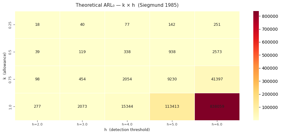
Figure 2: Siegmund theoretical ARL₀ across the full k × h grid. The theoretical surface grows extremely fast: at k = 1.00, h = 6.0 predicts over 838,000 bars between false alarms.

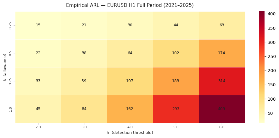
Figure 3: Empirical ARL₀ on EURUSD H1, full period 2021–2025. The empirical surface never exceeds 409 bars anywhere in the tested grid, including at the most conservative corner where theory predicts over 838,000.

The ratio of empirical to theoretical degrades steadily as h increases at fixed k = 0.50: 0.564 at h = 2, 0.321 at h = 3, 0.188 at h = 4, 0.109 at h = 5, and 0.067 at h = 6. The more conservative the threshold, the worse the formula’s relative accuracy becomes.

Key Finding 3

There is no value of h within the tested range that brings empirical behavior into line with Siegmund’s theoretical prediction on EURUSD H1. Practitioners calibrating this indicator for production use should select h empirically against their target instrument’s own historical breakpoint frequency, rather than relying on the closed-form ARL₀ formula to set expectations.

Detection Latency at Known Macro Events

On the Event Timestamps Used Below

The t₀ datetime for each event was identified by visually inspecting the relevant chart and selecting the bar judged to be the start of the directional impulse. These are analyst estimates tied to real, dated events — not the exact timestamp of the news release. Latency figures should be read as approximate indicators of detection speed, not precise measurements. 

Table 5 reports detection latency in bars for 21 event/instrument/timeframe combinations at h = 4.0, h = 5.0, and h = 6.0.

Symbol	TF	Event	t₀	h = 4.0	h = 5.0	h = 6.0
EURUSD	H1	EUR breakdown — Ukraine invasion	2022-02-24	4	4	4
EURUSD	H4	EUR breakdown — Ukraine invasion	2022-02-24	0	1	1
EURUSD	M15	EUR breakdown — Ukraine invasion	2022-02-24	17	17	17
EURUSD	H1	EUR drop — US election result	2024-11-06	130	132	293
EURUSD	H4	EUR drop — US election result	2024-11-06	15	184	184
GBPUSD	H1	GBP mini-budget crash	2022-09-23	5	5	5
GBPUSD	H4	GBP mini-budget crash	2022-09-23	1	2	2
XAUUSD	H1	Gold spike — Ukraine invasion	2022-02-24	156	193	3
XAUUSD	H4	Gold spike — Ukraine invasion	2022-02-24	14	12	0
XAUUSD	H1	Gold ATH breakout	2024-10-18	33	78	78
XAUUSD	H4	Gold ATH breakout	2024-10-18	56	79	79
DE40	H1	DAX gap down — Ukraine invasion	2022-02-24	0	0	943
DE40	H4	DAX gap down — Ukraine invasion	2022-02-24	7	10	1
USTEC	H1	NASDAQ selloff — Jackson Hole	2022-08-26	3	3	3
USTEC	H4	NASDAQ selloff — Jackson Hole	2022-08-26	1	1	2
USTEC	H1	NASDAQ gap up — US election	2024-11-06	9	9	9
USTEC	H4	NASDAQ gap up — US election	2024-11-06	2	2	2
USDJPY	H1	JPY BOJ intervention	2022-09-22	175	342	365
USDJPY	H4	JPY BOJ intervention	2022-09-22	0	0	0
USDJPY	H1	JPY carry unwind — BOJ hike	2024-07-31	4	4	4
USDJPY	H4	JPY carry unwind — BOJ hike	2024-07-31	1	1	18

Summary across 21 events — Median: 5 / 5 / 4 bars  |  Mean: 30.1 / 51.4 / 95.9 bars  |  Min: 0 / 0 / 0 bars  |  Max: 175 / 342 / 943 bars (for h = 4.0 / 5.0 / 6.0 respectively). Bold: DE40 H1 Ukraine invasion at h = 6.0 took 943 bars (≈ 39 trading days) to confirm. t₀ timestamps are analyst estimates anchored to documented macro events, not exact news release times.

Table 5: Detection latency (bars) from t₀ to first confirmed breakpoint, for 21 event/instrument/timeframe combinations across three threshold values.

At h = 4.0, the median detection latency across all 21 events is 5 bars and the mean is 30.1 bars. Eleven of the 21 events were confirmed within 5 bars or fewer; three confirmed at 0 bars (the very same bar the event began). The mean is pulled sharply above the median by a handful of slow outliers: the USDJPY BOJ intervention of September 2022 took 175 bars at h = 4.0, and the EURUSD US election drop of November 2024 took 130 bars. As threshold increases, the median stays stable (5, 5, and 4 bars at h = 4, 5, 6) but the mean climbs steeply to 51.4 and 95.9, driven by an increasing number of slow-to-resolve cases.

The most striking single observation in the study is the DE40 H1 reaction to the Ukraine invasion gap at h = 6.0: it took 943 bars — nearly 40 trading days — to confirm, because the initial gap-down bar pushed the accumulator close to but not over threshold, and the subsequent choppy consolidation slowly drained it back toward zero before the threshold was eventually crossed. The same event was confirmed on bar 0 at h = 4.0, illustrating the latency cost of conservative threshold settings as sharply as any single data point in the study.

Key Finding 4

Detection latency is highly event- and instrument-dependent, but the typical case — the median across 21 tested events — resolves within single-digit bars even though a small number of slow outliers pull the mean much higher. This means the indicator is generally fast for sharp, discontinuous events, but practitioners should not assume uniform speed: gradual regime transitions can take substantially longer to cross the threshold, and that delay grows quickly as h is set more conservatively.

Conclusion

In summary, the detector fires about five times more often than the Siegmund formula predicts. The excess is concentrated in volatile periods; in quiet markets it is slightly more conservative than theory. About half of detections coincide with variance shifts, while mean shifts are rare. Frequency is broadly stable across periods, but no tested k/h combination aligns empirical and theoretical ARL. Event latency is typically low, though some cases are slow—especially at higher h.

None of this makes the indicator unusable. It makes it a specific, well-characterized tool: a fast, cross-asset-consistent detector of volatility regime changes, whose false-alarm rate must be calibrated empirically per instrument rather than assumed from closed-form theory, and whose conservative-threshold settings trade a meaningful amount of detection speed for a reduction in false alarms that is smaller than the textbook formula implies. A trader who began Part 1 asking why their moving averages and ATR filters always seemed to confirm a regime change after the fact now has both a working implementation and an honest, data-backed account of exactly what that implementation does and does not guarantee — which is the only sound basis for deciding how to actually use it.

Program used in the article:

#	Name	Type	Description
1	CUSUM_Breakpoint.mq5	Custom Indicator	A two-sided CUSUM structural breakpoint detector operating on standardized log-returns. It plots both accumulators against ±h threshold boundaries in a dedicated subwindow and marks every declared breakpoint as a vertical line on the main chart.