Measuring What Matters (Part 3): The Reconstruction Engine — Validating Risk Footprints with Matrix Algebra

Introduction

Part 2 of this series ended with a striking number: 91.24%. That was the share of total portfolio variance held by Factor 1 in the eigenvalue spectrum — a single underlying driver, almost entirely Gold, consuming nine tenths of the portfolio's entire risk budget. The CovarianceMatrix class built in Part 2 produced that figure by calling the native MQL5 .Eig() method on the covariance matrix, which returned a set of eigenvectors V and eigenvalues λ that described the portfolio's risk in terms of independent, orthogonal factors.

But here is a question worth asking before building anything further on top of that decomposition: how do you know the eigenvectors and eigenvalues are correct? How do you know that the three factors extracted by .Eig() genuinely capture the complete risk structure of the portfolio — not an approximation of it, but its exact representation in exact arithmetic and its numerical equivalent within floating-point precision?

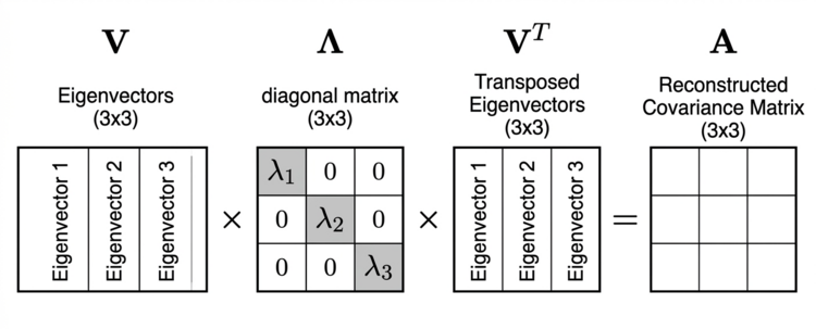
In pure mathematics, the answer comes from the spectral theorem. For any real symmetric matrix A — which a covariance matrix always is — the theorem guarantees that A can be exactly reconstructed from its eigenvectors and eigenvalues using the formula:

A = V Λ Vᵀ

Why does this matter practically? Because for a real symmetric covariance matrix, the full eigendecomposition is a lossless representation in exact arithmetic.

Where V is the matrix of eigenvectors (each column one eigenvector), Λ is a diagonal matrix with the eigenvalues on its main diagonal, and Vᵀ is the transpose of V. If the decomposition captured everything, then in exact arithmetic the triple product reconstructs the original matrix and the residual is zero. In floating-point computation, the residual should be close to zero, with any non-zero entries arising solely from rounding error and typically remaining near machine precision relative to the matrix scale. 

Part 3 demonstrates this numerically using a practical example. The practical project is EigenRecomposer.mq5. It reuses the covariance-matrix pipeline from Part 2, decomposes the matrix with .Eig(), builds Λ with Lambda.Diag(lambda), reconstructs A via V × Λ × Vᵀ using .MatMul() and .Transpose(), and computes the residual using MQL5's native matrix subtraction. The residual is then quantified using the Frobenius norm. The result is a numerical verification, printed directly to the Experts journal, that the spectral decomposition performed in Part 2 reconstructs the portfolio's covariance matrix with only floating-point rounding error.

Along the way, Part 3 teaches three new MQL5 matrix operations that will be used repeatedly in the parts that follow: Lambda.Diag() for constructing diagonal matrices, .Transpose() for matrix transposition, and .MatMul() for chaining matrix multiplications. Each one is introduced in the context where it is needed, explained precisely, and used immediately in working code.

What the Spectral Theorem Actually States

Before writing a single line of code, the mathematics of Part 3 deserves a clear statement in plain language.

The spectral theorem for real symmetric matrices says that any such matrix A can be decomposed as:

A = V Λ Vᵀ

Each term in this product has a specific meaning. V is the matrix whose columns are the eigenvectors of A, each column representing an orthogonal direction in the portfolio's asset space. Λ (Lambda) is a diagonal matrix — a square matrix where every off-diagonal entry is zero and the main diagonal holds the eigenvalues, each measuring the variance capacity of its corresponding factor direction. Vᵀ is simply V with its rows and columns swapped.

The theorem makes a strong claim: in exact arithmetic, this product reconstructs A exactly. In floating-point computation, any deviation arises solely from rounding error and is therefore expected to remain near machine precision relative to the matrix scale.

This matters because, for a real symmetric covariance matrix, the eigendecomposition is lossless in exact arithmetic. The original variances, covariances, and implied correlations are fully encoded by the three eigenvectors and three eigenvalues. Nothing is approximated or discarded during the decomposition itself. The eigendecomposition is not a simplification of the covariance matrix; in exact arithmetic, it is an exact alternative representation of it.

This guarantee is the mathematical foundation that makes eigenvalue-based portfolio analysis trustworthy. If the spectral theorem did not hold — if the decomposition were lossy — then any position sizing, concentration measurement, or stress test built on eigenvectors would be operating on incomplete information. The numerical reconstruction performed in this article verifies that MQL5's eigendecomposition satisfies this theoretical identity within floating-point precision, with the evidence printed directly to the journal.

The Script Structure: Eight Steps to a Numerical Verification

EigenRecomposer.mq5 is structured in eight sequential steps, each printed clearly to the journal so you can follow the mathematical pipeline from raw price data to numerical verification. The input parameters are three symbol names, a timeframe, and a lookback period:

#property copyright   "Measuring What Matters Series — Part 3"
#property link        ""
#property version     "1.00"
#property script_show_inputs

//--- Input parameters
input string           Symbol1      = "EURUSD";   // First symbol
input string           Symbol2      = "GBPUSD";   // Second symbol
input string           Symbol3      = "XAUUSD";   // Third symbol
input ENUM_TIMEFRAMES TF           = PERIOD_H1;   // Timeframe
input int              LookbackBars = 100;        // Lookback period (bars)

No portfolio weight inputs are included because neither constructing the covariance matrix nor performing the spectral reconstruction depends on how the trader allocates capital. The matrix is a property of the instruments, not of the position sizing.

The Data Foundation: ComputeLogReturns and PrintDivider

The first responsibility of the script is collecting price history and converting it into logarithmic return series — the correct statistical input for covariance computation. The ComputeLogReturns function handles this for any single symbol:

//+------------------------------------------------------------------+
//| Helper: Compute log returns                                      |
//+------------------------------------------------------------------+
bool ComputeLogReturns(const string symbol,
                       ENUM_TIMEFRAMES tf,
                       int bars,
                       vector &log_returns)
  {
   vector prices;
   if(!prices.CopyRates(symbol, tf, COPY_RATES_CLOSE, 1, bars + 1))
     {
      PrintFormat("ERROR: Could not copy rates for %s. Error: %d",
                  symbol, GetLastError());
      return false;
     }

   log_returns.Init(bars);

   for(int i = 0; i < bars; i++)
     {
      if(prices[i] <= 0.0 || prices[i + 1] <= 0.0)
        {
         PrintFormat("ERROR: Invalid price encountered for %s at index %d.",
                     symbol, i);
         return false;
        }

      log_returns[i] = MathLog(prices[i] / prices[i + 1]);
     }

   return true;
  }

The function downloads close prices using prices.CopyRates(), requesting bars + 1 prices to produce exactly bars return observations because each return requires both a current and a previous price. The data request starts at shift 1, ensuring that only completed bars are used. As a result, prices[0] is the most recently closed bar and prices[i+1] is the preceding (older) bar. The logarithmic return formula MathLog(prices[i] / prices[i+1]) therefore computes ln(P_t / P_{t-1}). Using only completed bars improves the stability and reproducibility of the covariance estimates by avoiding the still-forming current candle. Log returns are used rather than simple percentage returns because they are additive over time and have better statistical properties for covariance estimation.

The zero-price guard prevents silent division-by-zero errors on any edge-case bar. If an invalid price is encountered, the function immediately returns false, allowing the caller to terminate before any covariance calculations are performed with incomplete or invalid data. The log_returns vector is passed by reference, so the & avoids an expensive copy and allows the function to modify the vector in place.

The PrintDivider helper prints a row of repeated characters to the journal, used throughout the script to separate output sections for readability.

A Reusable Helper: PrintMatrixGrid

This script needs to print three different matrices to the journal — the original covariance matrix, the reconstructed matrix, and the residual. Rather than writing separate print logic for each, PrintMatrixGrid is a single helper that accepts any matrix, any label array, and a title string, and renders a clean labeled grid with one call:

//+------------------------------------------------------------------+
//| Helper: Print a matrix grid with symbol labels                   |
//+------------------------------------------------------------------+
void PrintMatrixGrid(const matrix &m, const string &labels[], int size,
                     string title)
  {
   PrintDivider("=");
   Print("  " + title);
   PrintDivider();

   string header = StringFormat("  %12s", "");
   for(int col = 0; col < size; col++)
      header += StringFormat("  %-16s", labels[col]);
   Print(header);
   PrintDivider();

   for(int row = 0; row < size; row++)
     {
      string line = StringFormat("  %-12s", labels[row]);
      for(int col = 0; col < size; col++)
         line += StringFormat("  %+.8f    ", m[row][col]);
      Print(line);
     }
   PrintDivider("=");
  }

The function signature takes the matrix as a const matrix & — a const reference meaning no copy is made and the function cannot modify the data. The labels array is also passed by const reference. Both are correct practice for any function that only needs to read its inputs.

The header loop builds a row of column labels, each left-aligned in a 16-character field using %-16s. The data loop then builds each row — a symbol label on the left followed by each cell value formatted as %+.8f with an explicit sign. Eight decimal places are used because covariance values between forex instruments are typically in the range of 1×10⁻⁷ to 1×10⁻⁸, and without sufficient decimal places they would print as zero. The explicit + sign ensures positive and negative entries are immediately distinguishable — important when the residual matrix is printed and every cell should be near zero with either sign.

A New Helper: FrobeniusNorm

The second new helper is FrobeniusNorm:

//+------------------------------------------------------------------+
//| Helper: Compute Frobenius norm of a matrix                       |
//| Frobenius norm = sqrt( sum of all squared elements )             |
//| Used to quantify the magnitude of the residual error matrix      |
//+------------------------------------------------------------------+
double FrobeniusNorm(const matrix &m, int size)
  {
   double sum = 0.0;
   for(int i = 0; i < size; i++)
      for(int j = 0; j < size; j++)
         sum += m[i][j] * m[i][j];
   return MathSqrt(sum);
  }

The Frobenius norm is a single number that measures the overall magnitude of a matrix — the matrix equivalent of a vector's length. It is computed by summing the squares of every element in the matrix and taking the square root of that sum. For a residual matrix whose entries are all near machine precision relative to the matrix scale, the Frobenius norm will likewise remain very small relative to the matrix scale.

The reason for computing the Frobenius norm alongside the maximum cell error is that it captures the total reconstruction error across all nine cells simultaneously. The maximum cell error tells you the worst single deviation. The Frobenius norm tells you the combined magnitude of all deviations. When both numbers are consistent with floating-point rounding, they provide strong numerical evidence that the reconstruction agrees with the original matrix within floating-point precision, both in every cell and in aggregate.

Steps 1 and 2: Collecting Returns and Building the Covariance Matrix

Step 1 collects log returns for all three symbols using a loop over ComputeLogReturns, storing each symbol's return vector in a dynamic array. Before constructing the return matrix, the script verifies that all three return vectors have identical lengths, ensuring that every asset contributes the same number of observations to the covariance calculation. Step 2 builds the covariance matrix using MQL5's native matrix .Cov() method. The layout requirement is critical: assets must be arranged as rows and observations as columns, because .Cov() treats each row as a separate variable. Transposing this layout would cause .Cov() to return a [Bars × Bars] matrix rather than the [Assets × Assets] covariance matrix we need.

//--- Step 2: Build covariance matrix (same matrix pipeline as Part 2)

//--- Verify that all return series have identical lengths
  if(returns[0].Size() != returns[1].Size() ||
     returns[0].Size() != returns[2].Size())
    {
     Print("ERROR: Return series have inconsistent lengths. Exiting.");
     return;
    }

  ulong columns = returns[0].Size();
  matrix all_returns;
  all_returns.Init(3, columns);
  for(int i = 0; i < 3; i++)
     all_returns.Row(returns[i], i);

  matrix cov_original = all_returns.Cov();

all_returns.Init(3, columns) allocates a matrix with 3 rows (one per asset) and columns columns (one per bar). The loop uses .Row() to place each symbol's return vector into its designated row. .Cov() then computes the full 3 × 3 covariance matrix where entry [i][j] holds the covariance between asset i and asset j.

The variable is named cov_original deliberately — this script produces three matrices (original, reconstructed, and residual) and clear naming prevents confusion throughout the pipeline. After a shape guard confirms the matrix is 3 × 3, PrintMatrixGrid renders it to the journal as the ground truth that the reconstruction must match exactly.

Step 3: Eigenvalue Decomposition

The native MQL5 .Eig() method decomposes the covariance matrix into its eigenvectors and eigenvalues in a single call:

//--- Step 3: Eigenvalue decomposition — .Eig()

   matrix V;       // Eigenvectors — each COLUMN is one eigenvector
   vector lambda;  // Eigenvalues  — lambda[k] matches column k of V

   if(!cov_original.Eig(V, lambda))
     {
      Print("ERROR: Eigenvalue decomposition failed. Exiting.");
      return;
     }

The parameter order is critical and fixed by the MQL5 API: eigenvectors first, eigenvalues second. After a successful call, V is a 3 × 3 matrix where each column is one eigenvector, and lambda is a vector of three eigenvalues where lambda[k] corresponds to column k of V. This column-to-eigenvalue pairing must be preserved throughout the reconstruction — it is the link that makes the spectral theorem work.

The variable names V and lambda are chosen to mirror the mathematical notation of the spectral theorem A = V Λ Vᵀ directly. When Step 5 writes V.MatMul(Lambda), the connection to the formula is immediate.

After decomposition, the script prints an eigenvalue summary:

//--- Print the eigenvalue summary
   double total_var = 0.0;
   for(int i = 0; i < (int)lambda.Size(); i++)
      total_var += lambda[i];

   Print("  Eigenvalue Summary:");
   for(int i = 0; i < (int)lambda.Size(); i++)
     {
      double pct = (total_var > 0) ? (lambda[i] / total_var) * 100.0 : 0.0;
      PrintFormat("  lambda[%d] = %+.8f  (%.2f%% of total variance)",
                  i, lambda[i], pct);
     }

The output uses lambda[%d] — the variable name from the code — rather than "Factor 1, 2, 3." This is deliberate: the eigenvalues have not been sorted from largest to smallest at this stage, so labeling them as factors would imply an ordering that does not yet exist. Printing them as lambda[0], lambda[1], lambda[2] is honest about what they are: unsorted raw outputs from the decomposition. Sorting is unnecessary here because the spectral theorem holds for any ordering — as long as column k of V always pairs with lambda[k], the triple product reconstructs the original matrix exactly.

Step 4: Constructing the Diagonal Matrix Lambda

This is the first genuinely new MQL5 operation introduced in Part 3, and it requires careful explanation because the correct usage differs from what many developers might initially expect.

//--- Step 4: Construct diagonal matrix Lambda from eigenvalue vector
//--- The spectral theorem requires Lambda as a square diagonal matrix
//--- where Lambda[i][i] = lambda[i] and all off-diagonal entries = 0
//--- NOTE: Diag() is a MATRIX method, not a vector method, and it is
//--- void — it fills the matrix in place rather than returning one.
//--- Called on an unallocated matrix, it auto-sizes to a square
//--- matrix matching the vector's length and places the vector's
//--- values on the main diagonal (all other entries become 0).
   Print("Step 4: Constructing diagonal matrix Lambda via Lambda.Diag(lambda)...");

   matrix Lambda;
   Lambda.Diag(lambda);

Diag() is a method of the matrix type, not a static factory function. It is called on a matrix object and takes a vector as its argument. It is also void — it does not return a new matrix; it fills the matrix it is called on in place. When called on an unallocated matrix (as Lambda is here, declared but not yet initialized), it automatically sizes itself to a square matrix whose dimension matches the vector's length and places the vector's values on the main diagonal. Every off-diagonal entry is set to zero. For our three-symbol case with lambda holding three eigenvalues, this produces a 3 × 3 diagonal matrix:

λ₀	0	0
0	λ₁	0
0	0	λ₂

The script prints this matrix explicitly so the reader can verify that the off-diagonal entries are exactly zero:

for(int i = 0; i < 3; i++)
   {
    string row_str = "    [ ";
    for(int j = 0; j < 3; j++)
       row_str += StringFormat("%+.8f  ", Lambda[i][j]);
    row_str += "]";
    Print(row_str);
   }

Seeing all six off-diagonal entries print as +0.00000000 confirms that Lambda.Diag(lambda) constructed the expected diagonal matrix. This is a small but important verification step because the spectral theorem represents the eigenvalues in a diagonal matrix. Any unintended off-diagonal entry would change the diagonal eigenvalue matrix and therefore alter the reconstructed covariance matrix.

Step 5: Executing the Spectral Theorem — V × Λ × Vᵀ

Step 5 is the mathematical core of Part 3. It executes the triple matrix product that the spectral theorem describes, in two sequential .MatMul() calls:

//--- Step 5: Reconstruct the covariance matrix using the spectral theorem
//--- A = V * Lambda * V^T
//--- Step A: Compute V * Lambda
//--- Step B: Compute (V * Lambda) * V^T
//--- Executed entirely using MQL5's native matrix algebra functions

   matrix V_transpose       = V.Transpose();            // V^T
   matrix VL                = V.MatMul(Lambda);         // V * Lambda
   matrix cov_reconstructed = VL.MatMul(V_transpose);  // (V * Lambda) * V^T

Three lines. Three matrix operations. Together they implement A = V Λ Vᵀ completely. Each line deserves precise explanation.

Line 1: V.Transpose()

.Transpose() is a method of the matrix type that returns a new matrix with rows and columns swapped. If V is a 3 × 3 matrix where column k is the k-th eigenvector, then V_transpose is the same matrix with each column becoming a row. The entry at [row][col] in V becomes the entry at [col][row] in V_transpose. The method creates a new matrix object and leaves V unchanged — which is important because V is needed in its original form for the next line.

Line 2: V.MatMul(Lambda)

.MatMul() performs standard matrix multiplication — the dot product of rows from the left matrix with columns from the right matrix. V.MatMul(Lambda) computes the product of the 3 × 3 eigenvector matrix with the 3 × 3 diagonal eigenvalue matrix. Because Lambda is diagonal, this multiplication has a specific geometric meaning: each column of V (each eigenvector) is scaled by its corresponding eigenvalue. Eigenvectors with large eigenvalues are stretched; eigenvectors with small eigenvalues are compressed. The result VL is an intermediate matrix that encodes both the directions (from V) and the magnitudes (from Λ) of the risk factors.

Line 3: VL.MatMul(V_transpose)

The second .MatMul() completes the reconstruction. Multiplying the intermediate VL by Vᵀ rotates the scaled eigenvectors back into the original coordinate system — the space where rows and columns represent EURUSD, GBPUSD, and XAUUSD rather than abstract factor directions. The result, cov_reconstructed, should be identical to cov_original within floating-point precision.

The chaining of .MatMul() calls is natural in MQL5 because each call returns a matrix object. The intermediate result VL could have been written inline: cov_reconstructed = V.MatMul(Lambda).MatMul(V_transpose). Writing it as two explicit lines with the named intermediate VL is a deliberate choice for readability — the reader can see each multiplication as a separate step, connecting to the formula A = V Λ Vᵀ one product at a time.

Step 6: The Residual — Native Matrix Subtraction

With both the original and reconstructed matrices in hand, computing the residual takes one line:

//--- Step 6: Compute residual matrix = Original - Reconstructed
//--- In exact arithmetic every cell is exactly zero.
//--- In floating-point arithmetic every cell should remain near the rounding-error scale.
//--- Optimized to use MQL5 native matrix operator subtraction.

   matrix residual = cov_original - cov_reconstructed;

This uses MQL5's native matrix subtraction operator. The - operator on two matrix objects performs element-wise subtraction — each cell of cov_original minus the corresponding cell of cov_reconstructed — and returns a new matrix of the same dimensions. No loop is needed. No manual indexing. The native operator handles it in a single expression. This is worth contrasting with how the same operation might have been written without the native operator:

//--- Manual approach — not used in this script
  for(int i = 0; i < 3; i++)
     for(int j = 0; j < 3; j++)
        residual[i][j] = cov_original[i][j] - cov_reconstructed[i][j];

Both produce identical results. The native operator version is shorter, reads closer to the mathematical notation (Original − Reconstructed), and benefits from the same OpenBLAS acceleration that underlies all native matrix operations. For a 3 × 3 matrix the performance difference is negligible, but the habit of using native operators over manual loops scales well as matrix sizes grow in later parts of this series.

After computing the residual, PrintMatrixGrid renders it with the title "RESIDUAL MATRIX (Original - Reconstructed)". Every cell in this grid should print as a value near machine precision relative to the matrix scale, making the residual indistinguishable from zero for practical purposes.

Steps 7 and 8: Quantifying the Error — Frobenius Norm and Max Cell Error

Two error metrics are computed from the residual matrix and reported together:

//--- Step 7: Frobenius norm of the residual — quantifies total error
   double frob_norm = FrobeniusNorm(residual, 3);

//--- Step 8: Max absolute cell error — finds the largest single deviation
   double max_error = 0.0;
   for(int i = 0; i < 3; i++)
     {
      for(int j = 0; j < 3; j++)
        {
         if(MathAbs(residual[i][j]) > max_error)
            max_error = MathAbs(residual[i][j]);
        }
     }

The Frobenius norm is computed by the helper function introduced earlier — summing squared elements and taking the square root. For a residual near machine precision relative to the matrix scale, the Frobenius norm is likewise expected to remain near that level.

The max cell error loop iterates every cell and tracks the largest absolute value found. This is the single worst deviation in the entire reconstruction — the cell where floating-point arithmetic accumulated the most rounding error. If the spectral theorem holds (which it will for a correctly computed covariance matrix), this value is likewise expected to remain near machine precision relative to the matrix scale. The final verdict uses the max cell error as the pass/fail criterion:

//--- Verdict: if max error < 1e-10 the reconstruction is numerically exact
   if(max_error < 1e-10)
      PrintFormat("  RESULT: Reconstruction agrees within floating-point precision. "
            "Max error = %.2e\n"
            "Reconstruction error is consistent with floating-point rounding only.",
            max_error);
   else
      PrintFormat("  WARNING: Reconstruction error exceeds expected threshold. "
                  "Max error = %.2e\n. Review data or decomposition.", max_error);

The threshold is 1×10⁻¹⁰: far above machine epsilon yet far below typical covariance magnitudes in this example. This gives the check ample room to pass in the presence of normal floating-point noise while still catching genuine reconstruction failures that would indicate a data layout error or a corrupted decomposition.

Reading the Output: What Three Matrices Tell You

When you run EigenRecomposer.mq5 with default inputs, the journal prints three matrix grids in sequence followed by the accuracy report. Reading them together tells a complete story about what the spectral theorem guarantees.

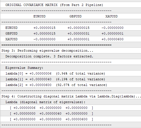
The first grid is the original covariance matrix — the ground truth computed directly from price data via .Cov(). For the EURUSD, GBPUSD, XAUUSD portfolio on H1 with a 100-bar lookback, the output shows:

                 EURUSD            GBPUSD            XAUUSD
EURUSD        +0.00000015       +0.00000015       -0.00000000
GBPUSD        +0.00000015       +0.00000031       +0.00000001
XAUUSD        -0.00000000       +0.00000001       +0.00000600

Several things stand out immediately. XAUUSD's own variance of +0.00000600 is by far the largest diagonal entry — forty times the size of EURUSD's variance and roughly twenty times GBPUSD's. This is the dominant feature of the risk structure. The EURUSD/XAUUSD entry is effectively zero (-0.00000000) meaning Gold and EURUSD moved nearly independently over this lookback window. The GBPUSD/XAUUSD entry is a tiny positive +0.00000001 — also negligible. The two currency pairs share a positive covariance of +0.00000015, equal to EURUSD's own variance, confirming they move together strongly. The eigenvalue summary printed just above confirms the structure: lambda[2] carries 92.87% of total portfolio variance, lambda[1] carries 6.19%, and lambda[0] carries only 0.94%.

The diagonal matrix Λ printed after the eigenvalue summary shows the three eigenvalues placed on the main diagonal with exact zeros everywhere else:

[ +0.00000006   +0.00000000   +0.00000000 ]
[ +0.00000000   +0.00000040   +0.00000000 ]
[ +0.00000000   +0.00000000   +0.00000600 ]

This is what Lambda.Diag(lambda) produced — a clean diagonal structure where every off-diagonal entry is exactly zero, confirming the method worked correctly before the triple matrix product is attempted.

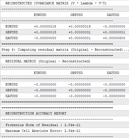
The second grid is the reconstructed covariance matrix — computed entirely from V, Λ, and Vᵀ with no reference to the original values during the calculation:

                EURUSD            GBPUSD            XAUUSD
EURUSD        +0.00000015       +0.00000015       -0.00000000
GBPUSD        +0.00000015       +0.00000031       +0.00000001
XAUUSD        -0.00000000       +0.00000001       +0.00000600

It is identical to the original at eight decimal places. Every value is preserved — including the effectively-zero EURUSD/XAUUSD entry and the tiny GBPUSD/XAUUSD entry of +0.00000001. The dominant +0.00000600 XAUUSD variance is reproduced exactly. The triple product V × Λ × Vᵀ reconstructed the original matrix within floating-point precision using only its eigenvectors and eigenvalues.

The third grid is the residual — the original minus the reconstructed:

                 EURUSD            GBPUSD            XAUUSD
EURUSD        -0.00000000       +0.00000000       -0.00000000
GBPUSD        +0.00000000       -0.00000000       -0.00000000
XAUUSD        -0.00000000       -0.00000000       +0.00000000

Every cell prints as ±0.00000000. At eight decimal places the residual is indistinguishable from zero in every cell. The accuracy report below it confirms the exact magnitude:

Frobenius Norm of Residual: 2.54e-21
Maximum Cell Absolute Error: 2.54e-21
RESULT: Reconstruction agrees within floating-point precision.
 Max error consistent with floating-point rounding only.

A maximum cell error of 2.54×10⁻²¹ is numerically negligible relative to the covariance values being analyzed and is consistent with ordinary floating-point rounding error. The smallest non-zero covariance value in the original matrix is +0.00000001 (the GBPUSD/XAUUSD covariance). The reconstruction error is thirteen orders of magnitude smaller than that. The Frobenius norm of 2.54×10⁻²¹ confirms this holds not just for the worst cell but across all nine cells simultaneously — both error metrics being equal here indicates the error is concentrated in one dominant cell, consistent with floating-point rounding behavior.

The numerical reconstruction confirms that this portfolio's covariance matrix satisfies the spectral theorem within floating-point precision. The three eigenvectors and three eigenvalues extracted by .Eig() encode the complete risk structure — every variance, every covariance, every near-zero entry — with no practically meaningful information loss.

What This Means for the Series

The numerical verification produced by this script is not just an academic exercise. It has a direct practical consequence for any analysis built on eigenvalue decomposition.

Any application that uses eigenvectors to compute position weights, measure risk concentration, or simulate stress scenarios is implicitly relying on those eigenvectors being a faithful, complete representation of the covariance structure. The numerical reconstruction provides strong evidence that they are — not merely as a theoretical claim but as a measured result for this example. For this portfolio, the maximum reconstruction error was 2.54×10⁻²¹, the Frobenius norm of the residual was also 2.54×10⁻²¹, and the reconstructed matrix matched the original at every decimal place the journal can display. The dominant +0.00000600 XAUUSD variance, the 92.87% concentration in lambda[2], the near-zero EURUSD/XAUUSD relationship — all of it was encoded in the eigenvectors and reconstructed within floating-point precision by the V × Λ × Vᵀ computation.

The three matrix operations introduced in this article — Lambda.Diag(), .Transpose(), and chained .MatMul() — are also fundamental tools in their own right. Having seen them used together in a context where correctness is independently verifiable (the residual should remain negligible within floating-point precision), you now have a concrete, tested understanding of how each operation behaves in MQL5 before applying them in more complex, less self-checking contexts.

The spectral theorem is not the destination of this series. It is the mathematical guarantee that everything built from eigenvalues is standing on solid ground.

Conclusion

Part 2 decomposed the covariance matrix into eigenvalues and eigenvectors and showed that the dominant factor held 91.24% of total portfolio variance. Part 3 numerically verifies that decomposition reconstructs the covariance matrix within floating-point precision. The dominant factor in Part 3's run shows 92.87% — slightly different from Part 2's 91.24% because both scripts were run on different market data windows; covariance structure is not static and shifts as new bars enter the lookback period.

EigenRecomposer.mq5 verifies the decomposition numerically. It builds Λ with Lambda.Diag(lambda), computes V × Λ × Vᵀ via .Transpose() and two .MatMul() calls, subtracts the result from the original matrix, and quantifies the residual using the Frobenius norm that the reconstructed covariance matrix agrees with the original within floating-point precision. The maximum reconstruction error was 2.54×10⁻²¹ and the Frobenius norm of the residual was also 2.54×10⁻²¹ — both thirteen orders of magnitude below the smallest meaningful covariance value — confirming the reconstruction differs from the original only by floating-point rounding error across all nine matrix entries.

The three new matrix operations introduced in this part — Diag(), .Transpose(), and .MatMul() — join CopyRates(), .Cov(), and .Eig() as the growing toolkit of native MQL5 linear algebra methods this series builds on. Each part introduces the operations it needs and uses them immediately in verifiable, runnable code.

In Part 4, we take the eigenvalue spectrum out of a verification script and into a live reading tool — examining what the distribution of eigenvalues across factors tells a trader about the current state of their portfolio's risk concentration, and building the metrics that will drive the indicator in Part 5.