The Avellaneda-Stoikov Model: Inventory-Aware Quoting for Two-Sided Strategies

Contents

1. Introduction
2. What you get
3. The model: reservation price and optimal spread
4. Estimating the inputs: volatility and order-flow intensity
5. The model class and its ground-truth check
6. Seeing the quotes live on a chart
7. The simulation lab: fixed vs adaptive quoting
8. What this is, and what it is not
9. Conclusion

Introduction

A market maker quotes two prices at once. It offers to buy at the bid and to sell at the ask, and it earns the spread between them. The job carries two risks that pull against each other. The first is inventory risk: if the bid keeps getting hit, you accumulate a long position, and a market that then trends against you turns that position into a real loss. The second is adverse selection: when the market moves fast, your resting quotes get picked off by traders who know more than your stale prices do.

Fixed, symmetric quotes ignore both problems. A grid that places a buy limit and a sell limit the same distance from the mid, over and over, has no memory of how much inventory it is holding and no sense of how volatile the market has become. In a quiet range, the grid works. In a trend it loads up on one side and gets run over.

Marco Avellaneda and Sasha Stoikov solved this in their 2008 paper High-frequency trading in a limit order book. They derived, in closed form, exactly where to place the bid and the ask so that the two risks stay balanced: the fair price shifts against your inventory to encourage you back to flat, and the spread widens with volatility and thins with liquidity. The result is two short formulas that any developer can compute on every tick.

This article implements the formulas as a small, testable MQL5 library. It connects them to live volatility and order-flow estimates, plots the resulting quotes on the chart, and runs a controlled simulation against fixed quotes on real historical data. The reader who follows along gets a reusable model class, a visual indicator, and a backtest script that measures the difference.

One important limitation upfront: a retail MetaTrader 5 account is a price taker, not an exchange market maker. Therefore, this does not promise that you can earn the spread by quoting both sides. Read it instead as two practical things: a simulation lab for studying inventory control, and a principled way to decide where a two-sided strategy should place its limit orders.

What you get

Before any theory, here is the payoff. The core of the article is a simulation that runs two market makers over the same 5000 bars of EURUSD H1 history. Both quote a bid and an ask on every bar. One uses a fixed 100-point spread with no inventory awareness. The other uses the Avellaneda-Stoikov quotes. The script reports the inventory each one carried and the profit and loss each one ended with.

Strategy	Buys / Sells	Final inventory (lots)	Max abs inventory	Inventory std	P&L
Fixed spread	2198 / 2152	4.60	5.10	1.405	-3145.20
Avellaneda-Stoikov	1661 / 1658	0.30	1.20	0.411	710.52

The fixed maker drifted to more than four lots long and stayed there, and it finished the run down. The Avellaneda-Stoikov maker held its inventory near zero the whole time, cutting the inventory standard deviation by 70.8 percent. The four figures below plot both makers over the same run.

Inventory in lots. The red fixed-spread line wanders between two and five lots, while the blue Avellaneda-Stoikov line stays pinned near zero.

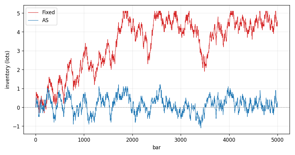
Fig. 1. Inventory in lots over 5000 bars of EURUSD H1. The fixed-spread maker (red) drifts to four or five lots, while the Avellaneda-Stoikov maker (blue) holds its inventory near zero.

Equity in account currency. The fixed maker's curve swings violently and ends negative, while the adaptive maker's curve is nearly flat and slightly positive.

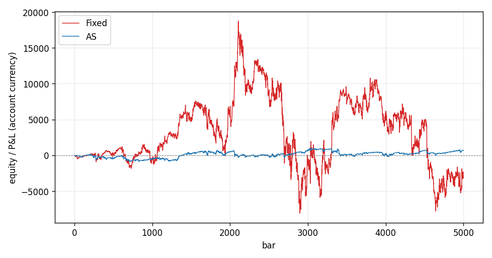
Fig. 2. Equity in account currency. The fixed-spread maker (red) swings violently and ends negative, while the Avellaneda-Stoikov maker (blue) stays nearly flat and slightly positive.

The last two figures show the model itself at work. The optimal spread widens in volatile stretches and thins when the market is calm.

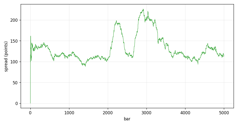
Fig. 3. The Avellaneda-Stoikov optimal spread in points. It widens in volatile stretches and thins when the market is calm.

The inventory skew leans the fair price up and down to push the position back toward zero.

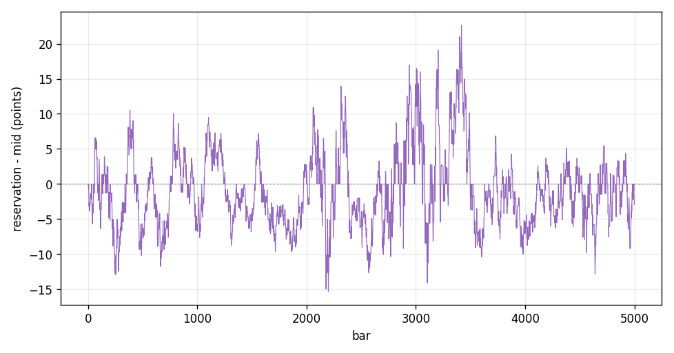
Fig. 4. The Avellaneda-Stoikov inventory skew, the reservation price minus the mid, in points. It leans the fair price up and down to push inventory back toward zero.

That is what this article delivers. The rest explains how, starting with the two formulas at the center of it.

The model: reservation price and optimal spread

Avellaneda and Stoikov start from a single insight. The price you quote around should not be the mid price. It should be a reservation price, the mid price shifted against your current inventory. If you are long, you want to sell more than you buy, so your fair price should sit a little below the mid to make your ask more attractive and your bid less so. The shift grows with how much inventory you hold, how risk averse you are, how volatile the market is, and how long you still intend to trade.

r = mid - q * gamma * sigma^2 * (T - t)

Here q is the signed inventory (positive when long), gamma is a risk-aversion constant, sigma is the volatility of the mid price, and (T - t) is the time left in the trading horizon. When q is zero the reservation price is just the mid. When q is positive the whole term is subtracted, pulling the fair price down so the position naturally unwinds.

Two of these inputs are worth slowing down on, because they are the knobs you actually turn. Gamma is how much the maker fears inventory. Set it near zero and the inventory term almost vanishes: the reservation price barely moves off the mid, the maker quotes symmetrically, and it will happily accumulate a large position. Raise gamma and every open lot pushes the fair price harder against itself, so the maker fights its own inventory sooner and holds a tighter position at the cost of quoting less competitively. There is no single correct value. It is a preference for flat inventory over captured spread, and the right setting depends on how much position risk you are willing to carry.

The horizon (T - t) is the second knob, and it is the one that trips people up. It is the number of steps left before the maker expects to be done trading, measured in the same units the estimator is fed. On a bar-by-bar feed it is a count of bars. Both the inventory shift and the volatility part of the spread scale directly with it, so a horizon of one bar makes the inventory skew almost invisible, while a horizon of a few hundred bars makes it large enough to steer real position control. It represents a holding period, not a magic constant, and it has to be chosen to match the strategy that consumes the quotes.

The second formula sets the total spread around that reservation price.

delta = gamma * sigma^2 * (T - t) + (2 / gamma) * ln(1 + gamma / k)

The spread has two parts. The first term is the same volatility-and-horizon product from the reservation price: the more the market can move before your horizon ends, the wider you quote to protect yourself. The second term depends on k, the intensity of order flow. A large k means orders arrive close to the mid and fills are easy, so you can quote tight; a small k means you must reach further out for a fill, so the spread widens. The quotes then straddle the reservation price:

bid = r - delta / 2 and ask = r + delta / 2

The picture below lays the four prices on a single axis. The mid sits in the center. The reservation price is pulled to one side by the inventory, here a long position pushing it below the mid. The bid and the ask then straddle the reservation, not the mid, so the whole quote leans toward the side that unwinds the position.

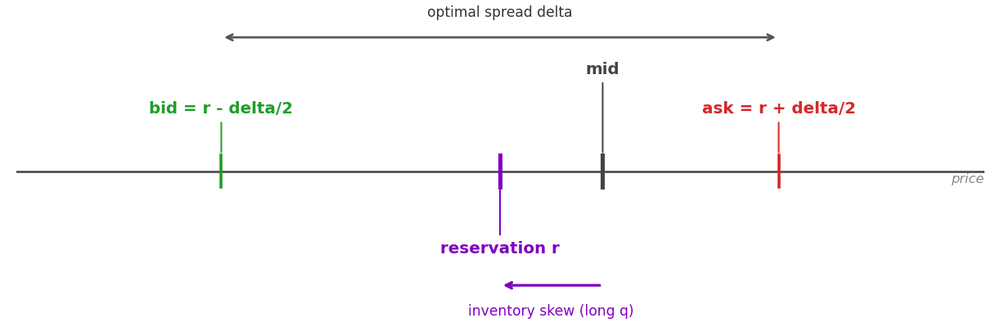
Fig. 5. A long inventory pulls the reservation price below the mid; the bid and ask then straddle the reservation, not the mid, so the whole quote leans toward the side that unwinds the position

These two lines are the entire model. The MQL5 class that computes them takes gamma as its one stored parameter and receives sigma, k, q, and the time left from the caller, which keeps the math pure and easy to test. The two closed-form results are one method each.

//+------------------------------------------------------------------+
//| r = mid - q * gamma * sigma^2 * (T - t)                          |
//+------------------------------------------------------------------+
double CAvellanedaStoikov::ReservationPrice(double mid, double q,
      double sigma, double timeLeft) const
  {
   return mid - q * m_gamma * sigma * sigma * timeLeft;
  }

//+------------------------------------------------------------------+
//| delta = gamma*sigma^2*(T-t) + (2/gamma)*ln(1 + gamma/k)          |
//+------------------------------------------------------------------+
double CAvellanedaStoikov::OptimalSpread(double sigma, double k,
      double timeLeft) const
  {
   double inventoryTerm = m_gamma * sigma * sigma * timeLeft;
   double liquidityTerm = (k > 0.0)
                        ? (2.0 / m_gamma) * MathLog(1.0 + m_gamma / k)
                        : 0.0;
   return inventoryTerm + liquidityTerm;
  }

The liquidity term guards against a zero or negative k, which the estimator can briefly return before it has seen enough data. When that happens the spread falls back to the volatility term alone rather than dividing by zero. A single Compute call wraps both formulas and fills a small result struct with the reservation price, the spread, and the two quotes.

//+------------------------------------------------------------------+
//| Reservation price + spread + bid/ask in one struct               |
//+------------------------------------------------------------------+
bool CAvellanedaStoikov::Compute(double mid, double q, double sigma, double k,
                               double timeLeft, ASQuote &out) const
  {
   if(m_gamma <= 0.0 || sigma < 0.0 || timeLeft < 0.0)
      return false;
   out.reservation = ReservationPrice(mid, q, sigma, timeLeft);
   out.spread      = OptimalSpread(sigma, k, timeLeft);
   out.bid         = out.reservation - 0.5 * out.spread;
   out.ask         = out.reservation + 0.5 * out.spread;
   out.skew        = out.reservation - mid;
   return true;
  }

The struct also stores the skew, the difference between the reservation price and the mid. It is not needed to place a quote, but it is exactly the quantity we want to plot later to see the inventory shift with the eye. The class is now complete, but it is only as good as the sigma and k we feed it. Those come next.

Estimating the inputs: volatility and order-flow intensity

The model needs two live numbers: sigma, the volatility of the mid price, and k, the intensity of order flow. Both are estimated from a rolling window of recent mid prices. The estimator takes one mid price at a time, turns it into an increment against the previous mid, and keeps running sums so that every query stays O(1) no matter how large the window.

Sigma is the standard deviation of those increments. The k term needs more thought. In the model, order flow arrives with an intensity that decays exponentially with distance from the mid, lambda(d) = A * exp(-k * d). We have no exchange order book on a retail feed, so we use a proxy: if move sizes are exponentially distributed, the maximum-likelihood estimate of the decay rate k is one divided by the mean absolute move. A market that moves in small steps has a large k and a tight spread; a market that lurches has a small k and a wide one. That is the behavior we want.

This estimate equals the reciprocal of the mean. This is also where the retail proxy departs from the original model. An exponential distribution with rate k has a mean of 1 / k. Turn that around and the rate is 1 / mean. So if you believe your price increments are drawn from that distribution, the single number that best fits it is the reciprocal of their average absolute size, and no windowed sum beyond the mean of the absolute moves is needed. That is why the estimator carries a running sum of absolute increments alongside the sum and the sum of squares: those three sums are all it takes to serve sigma and k on demand.

The gap to be honest about is the swap we made underneath. The real Avellaneda-Stoikov k describes how fill probability decays with quote distance in a limit order book, fitted to executed order flow. We have neither the book nor the fills, so we read k off the size distribution of price moves instead. The two are not the same quantity. What saves the substitution is that it moves in the right direction: a calm tape with small moves reports a large k and the spread tightens, a violent tape with large moves reports a small k and the spread widens. It is a behaviorally correct stand-in, not an exact reconstruction, and the article treats it as exactly that.

The heart of the estimator is a ring buffer that inserts each new increment and evicts the oldest when the window is full, adjusting the running sums as it goes.

//+------------------------------------------------------------------+
//| Insert one increment, evicting the oldest when the ring is full  |
//+------------------------------------------------------------------+
void CASEstimators::PushDelta(double d)
  {
   if(m_count >= m_cap)
     {
      double old = m_delta[m_head];
      m_sum    -= old;
      m_sumSq  -= old * old;
      m_sumAbs -= MathAbs(old);
     }
   else
      m_count++;
   m_delta[m_head] = d;
   m_sum    += d;
   m_sumSq  += d * d;
   m_sumAbs += MathAbs(d);
   m_head    = (m_head + 1) % m_cap;
  }

Because the sums are maintained incrementally, the two queries are trivial. The variance is the mean of the squares minus the square of the mean, clamped at zero to absorb floating-point noise on a flat window. The intensity is one over the mean absolute move, guarded so a flat window returns zero rather than dividing by zero.

//+------------------------------------------------------------------+
//| Population variance of the increments in the window              |
//+------------------------------------------------------------------+
double CASEstimators::Variance() const
  {
   if(m_count < 1)
      return 0.0;
   double mean = m_sum / m_count;
   double var = m_sumSq / m_count - mean * mean;
   return (var > 0.0 ? var : 0.0);
  }

//+------------------------------------------------------------------+
//| k = 1 / mean(|increment|), guarded against a flat window         |
//+------------------------------------------------------------------+
double CASEstimators::Intensity() const
  {
   double m = MeanAbsMove();
   if(m <= 0.0)
      return 0.0;
   return 1.0 / m;
  }

The estimator is deliberately agnostic about what a mid price is. Fed one tick mid at a time it produces tick-scale volatility; fed one bar close at a time it produces bar-scale volatility. The indicator uses the second form so that the quotes are visible on a normal chart, and the backtest uses the same to compare strategies bar by bar.

The model class and its ground-truth check

A two-line model is easy to get subtly wrong: a squared sigma that should not be squared, a sign flipped on the inventory term, a log argument off by one. The way to trust it is to compute a handful of cases by hand and assert the code matches. The self-check script does exactly that, with a small helper that compares a computed value to an expected one within a tolerance and tallies the result.

//+------------------------------------------------------------------+
//| Assert two doubles equal within tol; log PASS/FAIL               |
//+------------------------------------------------------------------+
void Check(string name, double got, double want, double tol = 1e-6)
  {
   if(MathAbs(got - want) <= tol)
     {
      g_pass++;
      PrintFormat("[PASS] %-28s got=%.8f", name, got);
     }
   else
     {
      g_fail++;
      PrintFormat("[FAIL] %-28s got=%.8f want=%.8f", name, got, want);
     }
  }

The expected values are worked out on paper. With gamma = 0.1, a mid of 100, an inventory of five lots, sigma = 2 and (T - t) = 1, the reservation price is 100 - 5 * 0.1 * 4 * 1 = 98.0. With k = 0.1 the spread is 0.1 * 4 * 1 + (2 / 0.1) * ln(1 + 1) = 0.4 + 20 * ln(2). The script checks these, checks that a long inventory pushes the reservation below the mid and a short inventory above it, and feeds the estimator known increment streams to confirm sigma and k. Running it prints a single summary line:

=== RESULT: 25 PASS, 0 FAIL ===

The full run is easier to read in the Experts log, one line per case, the model checks first and the estimator checks after.

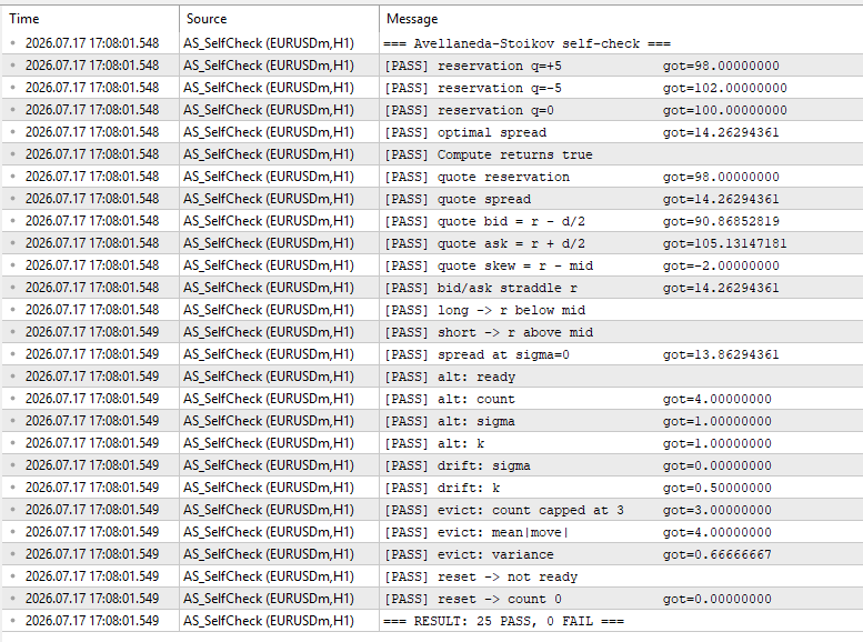
Fig. 6. The Experts log after running AS_SelfCheck, one PASS line per case and the final 25 PASS, 0 FAIL summary

Every case passes to within one part in a million. That rules out the sign, squaring, and off-by-one mistakes that a two-line model invites, and it means the numbers the rest of the article reports come from a model that is provably computing the formulas it claims to.

Seeing the quotes live on a chart

Numbers in a log are hard to trust until you see them move. The indicator plots three lines on the chart, the reservation price and the two quotes, and refreshes them on every tick. On each pass it recomputes the band over the recent bars: it feeds bar closes into the estimator, and once the estimator is ready it asks the model for a quote and writes the three values into the plot buffers. The core of that pass is the loop below, excerpted from OnCalculate; the surrounding setup, buffer allocation, and panel code are in the attached indicator.

for(int i = feedStart; i < rates_total; i++)
    {
     double mid = close[i];
     if(i == rates_total - 1 && liveMid > 0.0)
       mid = liveMid;
     g_est.AddMid(mid);
     if(i < drawStart || !g_est.Ready())
       continue;
     double sigma = g_est.Sigma();
     double k     = g_est.Intensity();
     ASQuote qt;
     if(!g_model.Compute(mid, q, sigma, k, InpTimeLeft, qt))
       continue;
     BufRes[i] = qt.reservation;
     BufBid[i] = qt.bid;
     BufAsk[i] = qt.ask;
     if(i == rates_total - 1 && InpShowInfo)
       PanelUpdate(sigma, k, q, qt);
    }

The last bar is special: it is still forming, so instead of its close the loop uses the live mid taken from the current bid and ask. The recompute walks a warm-up stretch before the drawn region so the estimator is already full by the time the first plotted bar is reached. The inventory q is read once per pass, either from a manual input or from the live net position on the symbol, so the reservation line can be watched shifting as a position is opened.

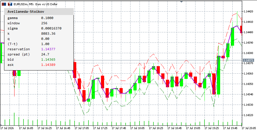
Fig. 7. The AS_Quotes indicator on EURUSD H1: the reservation line and the bid and ask band hug the price, with the status panel reporting sigma, k, the reservation, and the spread

On a EURUSD H1 chart a typical reading is a reservation price of 1.14335, a sigma of 0.00069, a k near 2004, and an optimal spread of about 100 points. The band hugs the price closely, which is exactly right: a real market maker's spread is small. The point of the plot is not a wide channel but a visible, adaptive one, tightening and widening with the market and, when inventory is present, leaning to one side.

The lean is easiest to see with a position on. Feed the indicator a few long lots through the manual inventory input and the whole band drops below the mid: the reservation line leads it down, the ask comes closer to the price to make selling easier, and the bid backs away. That is the inventory skew from the model made visible, the same shift the backtest exploits in the next section to keep its position near flat.

The simulation lab: fixed vs adaptive quoting

The indicator shows what the quotes look like. It does not show what they do. To measure that, the backtest script runs a full market-making loop over historical bars twice, once with a fixed spread and once with the model, and records the inventory and equity of each. Both runs share one function; a mode flag decides how the quotes are set.

The fill model is simple and the same for both strategies. On each bar, any quote resting from the previous bar is checked against the bar range: if the low reached the buy price, a buy fills and inventory rises; if the high reached the sell price, a sell fills and inventory drops. Then the estimator is updated with the new close and fresh quotes are set for the next bar. The only difference between the two strategies is those three lines that set the quotes.

Two aspects of this fill rule make the comparison fair. It fills a side only if the bar's range actually touched that quote, so neither strategy gets free fills, and it allows at most one buy and one sell per bar, so a single wide bar cannot load an unlimited position in one step. It is intentionally optimistic in one way: a real resting limit order competes for queue priority and can be skipped even when the price trades through it, which this loop ignores. That optimism is applied identically to both makers, so it cannot explain the difference between them. Both live under the same idealized fills and the same inventory cap; only the quote placement changes.

This makes the outcome depend only on the quoting rule. The fixed maker centers a constant band on the mid and has no memory of its position, so in a sustained trend the price keeps reaching one side of that band and skipping the other. It fills buy after buy on the way down, or sell after sell on the way up, and the inventory ratchets in one direction with no force pulling it back. The adaptive maker starts from the same fills but reacts to them: each lot it takes on shifts the reservation price against the position, which drags the opposite quote closer to the market and makes the unwinding fill easier to get. The position is therefore mean-reverting by construction, and the inventory curve stays pinned near zero instead of drifting.

The loop below is the heart of RunSim, excerpted to the fill-and-quote step; the setup, the statistics, and the CSV export around it are in the attached script.

for(int i = 0; i < n; i++)
    {
     //--- fill pending quotes against this bar's range
     if(haveQuote)
       {
        if(low[i] <= pendBid && q < maxInv)
          { q += InpLot; cash -= pendBid * InpLot; r.buys++; }
        if(high[i] >= pendAsk && q > -maxInv)
          { q -= InpLot; cash += pendAsk * InpLot; r.sells++; }
       }
     //--- record state after this bar's fills
     invOut[i] = q;
     eqOut[i]  = (cash + q * close[i]) * contract;
     //--- update estimator, then set quotes for the next bar
     est.AddMid(close[i]);
     if(!est.Ready())
       continue;
     double sigma = est.Sigma();
     double k     = est.Intensity();
     double mid   = close[i];
     if(mode == MM_FIXED)
       {
        pendBid = mid - halfFix;
        pendAsk = mid + halfFix;
       }
     else
       {
        ASQuote qt;
        if(!model.Compute(mid, q, sigma, k, InpTimeLeft, qt))
          continue;
        pendBid = qt.bid;
        pendAsk = qt.ask;
       }
     haveQuote = true;
    }

The fixed strategy centers a constant half-spread on the mid, forever. The adaptive strategy asks the model for its quotes, and because the model receives the current inventory q, its bid and ask shift against the position. That single difference produces the whole result in the table from the start of the article. The fixed maker has no mechanism to shed inventory, so in any trend it fills repeatedly on one side and rides the position; its equity swings with the market. The adaptive maker's reservation price leans away from its inventory, so its opposite quote gets easier to fill and the position mean-reverts to flat.

Both runs are written to a CSV, and a short Python script draws the four-panel figure shown earlier. The script's own summary confirms the MQL5 numbers exactly, an inventory standard deviation of 1.405 lots for the fixed maker against 0.411 for the adaptive one, which is the 70.8 percent reduction. The equity panel is the honest part of the story. The adaptive maker did finish this particular run ahead, but the message is not the profit. It is the flatness: the model traded away the wild equity swings of the fixed maker in exchange for control.

What this is, and what it is not

The result is clean, so it is worth being precise about its limits. Three points matter.

The first is the horizon term. The inventory shift and the volatility part of the spread both scale with (T - t). Measured on tick or bar volatility, that term is tiny unless the horizon is set to a meaningful number of steps. The examples here use a horizon of 600 bars, which is what makes the inventory skew large enough to matter and ties the model to a holding period a swing or grid strategy would actually run. Change the horizon and gamma together and the aggressiveness of the inventory control changes with them. These are tuning knobs, not universal constants.

The second is the k proxy. A real Avellaneda-Stoikov implementation fits k to executed order flow in a limit order book. A retail feed has none of that, so k here is inferred from the size distribution of price moves. It is a reasonable stand-in and it behaves correctly, tightening the spread in calm markets and widening it in violent ones, but it is an approximation, and the article does not pretend otherwise.

The third is the largest. A retail MetaTrader 5 account cannot actually be the maker that earns this spread. The simulation captures a modeled spread that a genuine exchange market maker would earn; you and I, quoting through a broker, are on the other side of that trade. So the honest use of this code is not a promise of free spread. It is a lab for studying how inventory-aware quoting controls risk, and a rule for where a two-sided limit-order strategy should place its orders. Read as that, the 70.8 percent figure is a real, reproducible property of the method, not a trading result.

It helps to be concrete about where the modeled spread goes. On an exchange, the market maker posts resting bids and asks and other participants cross the spread to trade against them, so the maker collects the difference as a rebate and a favorable fill. A retail order routed through a broker is on the taking side: your execution price already includes the broker's spread. Also, there is no exchange queue where your limit order can earn a rebate. The backtest's positive P&L is the spread the modeled maker captured in the simulation, and it does not survive being ported to a live retail fill. This is not a flaw in the code, it is the difference between simulating a role and occupying it.

What does survive the port is the inventory control itself. The reservation-price skew is a pure function of your current position, your risk aversion, and the measured volatility, and none of those depend on being an exchange maker. A grid, a scalper, or any two-sided strategy running on a retail account can compute the same skew and use it to decide where to place its next limit order, so that the placement leans against whatever inventory it is already carrying. That is the transferable part: not the spread, but the rule for where the orders go.

Important: The numbers in this article come from a single representative run on EURUSD H1. They demonstrate the model's behavior, not a forward-looking edge. Run the backtest on your own symbols and periods before drawing any conclusion, and treat the code as a research and order-placement tool rather than a live market-making system.

Conclusion

The Avellaneda-Stoikov model reduces to two short formulas, and this article turned them into a small MQL5 library you can compute on every tick. The reservation price leans against your inventory to pull it back to flat, and the optimal spread widens with volatility and thins with liquidity. Fed by rolling estimates of sigma and k, verified against hand-computed cases, drawn live on the chart, and measured in a controlled simulation, the model cut inventory standard deviation by 70.8 percent against a fixed-spread maker on the same history.

What was built:

• CAvellanedaStoikov, a pure-math class computing the reservation price, the optimal spread, and the two quotes.
• CASEstimators, an O(1) rolling estimator of volatility and order-flow intensity from mid prices.
• A self-check script that asserts the model against hand-computed values, passing all 25 cases.
• An indicator that draws the reservation price and the bid and ask band live on the chart.
• A backtest script that pits fixed quoting against adaptive quoting and exports the curves, with a Python plot to visualize them.

#	Filename	Type	Description
1	AvellanedaStoikov.mqh	Include	The model: reservation price, optimal spread, and the quote struct
2	ASEstimators.mqh	Include	Rolling O(1) estimators for volatility and order-flow intensity
3	AS_SelfCheck.mq5	Script	Ground-truth checks of the model and estimators against hand-computed values
4	AS_Quotes.mq5	Indicator	Draws the reservation price and the bid and ask band on the chart
5	AS_Backtest.mq5	Script	Simulates fixed vs adaptive quoting and exports the inventory and equity curves
6	as_plot_split.py	Python	Plots the four comparison figures (inventory, equity, spread, and skew) from the exported CSV