How to implement AutoARIMA forecasting in MQL5

Introduction

You want a practical one-step-ahead price forecast directly in the trading terminal, but ARIMA workflows create two common barriers: manual selection of p, d, and q and statistically robust parameter estimation that is awkward to embed in MQL5. This work addresses that engineering problem by providing a compact, reproducible procedure that accepts a single MQL5 array of recent closes (Close[0] = most recent) and returns a numeric forecast for the next close.

The implemented approach automates the full pipeline:

• (1) estimate differencing order d with a variance-based heuristic and apply differencing to obtain stationarity,
• (2) fit ARMA(p,q) models for a small grid of orders using SSE minimization with gradient-based updates and the Adam optimizer (coefficients clipped for stability),
• (3) select the best model by corrected AIC (AICc),
• and (4) invert differencing and round to tick size to produce a one-step price forecast.

Default limits (e.g., max p/max q = 5) and the one-step scope are explicit engineering choices to keep the routine reliable and fast for real-time use.

Time Series

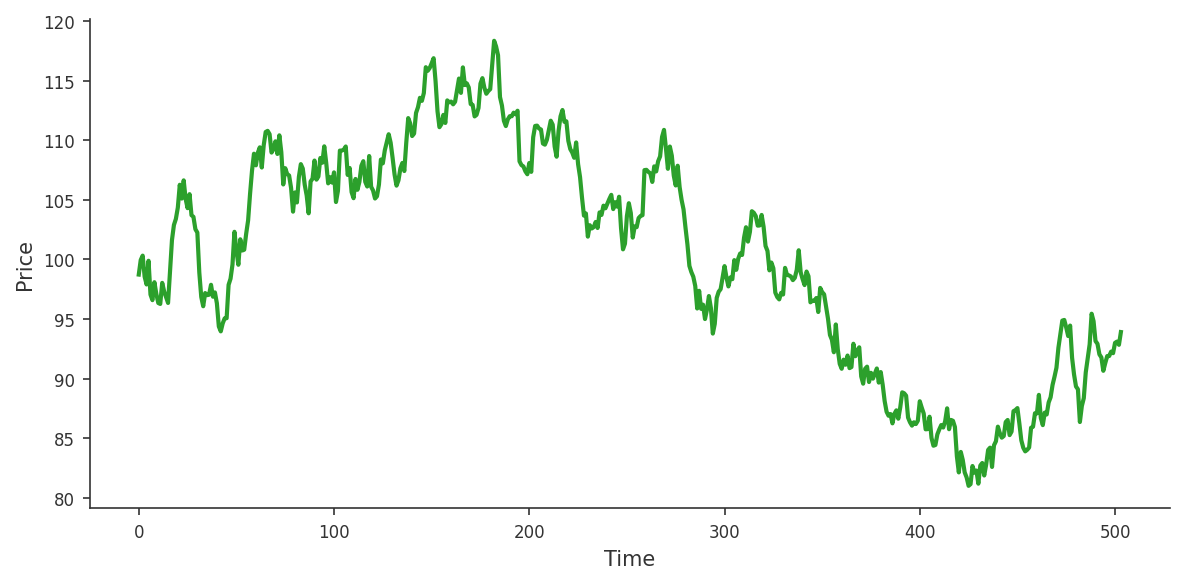
A time series is a sequence of observations indexed in time. Unlike traditional datasets, time series data may exhibit temporal dependence, where past values influence future observations. This dependency is not guaranteed, but when present, it provides the foundation for forecasting models such as ARIMA.

Financial prices are a time series: each candle close is assigned to a specific time, forming a sequence of observations ordered chronologically.

More generally, a time series can be written as a sequence:

Where each observation is indexed by time.

ARIMA

An ARIMA model is defined by three parameters: p, d, and q. Parameter p is the autoregressive order, d is the differencing order, and q is the moving-average order.

Parameter d

The parameter d plays a crucial role in transforming the series into a stationary process. Consider a time series that appears largely random, where prices can move up or down unpredictably. This behavior is typical of a non-stationary series: its statistical properties, such as the mean and variance, change over time.

This transformation measures the change between consecutive observations. If the original series exhibits a trend, the differenced series will often behave more like a stationary process.

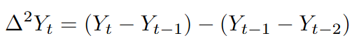
When the first difference is not sufficient, we difference the series twice:

Parameter p

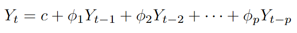
The parameter p defines the autoregressive component of the ARIMA model. This component captures the relationship between the current value of the series and its past observations. In other words, it assumes that the present can be partially explained by the past.

For example, in financial time series, it is common to observe short-term dependencies, where recent price movements influence the next ones. The autoregressive term models this behavior by assigning weights to previous values in the series.

As the value of p increases, the model incorporates a larger number of past observations, allowing it to capture more complex temporal structures. However, choosing a value that is too large may lead to overfitting, where the model starts to capture noise instead of meaningful patterns.

In essence, the autoregressive component answers a simple question: how much of the present can be explained by the past?

This is what an AR(p) looks like:

Errors (εₜ)

Before introducing the parameter q (moving average component), it is important to define the concept of an error in time series modeling.

In this context, an error (or residual) represents the difference between the observed value and the value forecasted by the model at a given time step. It can be expressed as

Where Yₜ is the observed (real) value and Ŷₜ is the forecasted value.

These errors capture the part of the series that the model is unable to explain.

Parameter q

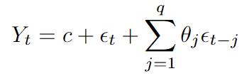
This parameter determines how many past errors are used to model the current value of the series. In practice, the moving-average component incorporates past forecast errors into the current estimate. If the model has consistently overestimated or underestimated recent values, the inclusion of past errors helps adjust future predictions accordingly.

This is what an MA(q) looks like:

ARMA(p,q)

After transforming the series to stationarity, we fit an ARMA model that combines autoregressive and moving-average terms. This model incorporates p past values of the series and q past errors and can be expressed as follows:

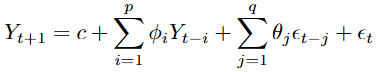
After this brief introduction to ARIMA models, a natural question arises: how do we choose the optimal values of p, d, and q?

This is precisely what AutoARIMA is designed to do: given a dataset, it automatically selects the best model and provides a forecast for the next time period.

Mean

Throughout the code, the mean of a time series is used as part of the model estimation process. It is defined as follows:

//+------------------------------------------------------------------+
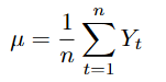
//| mean: arithmetic mean of a double array                          |
//+------------------------------------------------------------------+
double mean(const double &series[])
  {
   double sum = 0.0;
   int n = ArraySize(series);

   if(n == 0)
      return 0.0;

   for(int i=0;i<n;i++)
     {
      sum += series[i];
     }
   sum /= n;

   return sum;
  }

Variance

Also, the variance of a time series is used as part of the model estimation process. It is defined as follows:

//+------------------------------------------------------------------+
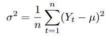
//| variance: population variance of a double array                  |
//+------------------------------------------------------------------+
double variance(const double &series[])
  {
   double sum = 0.0;
   int n = ArraySize(series);

   if(n < 2)
      return 0.0;

   double mu = mean(series);

   for(int i=0;i<n;i++)
     {
      sum += (series[i]-mu)*(series[i]-mu);
     }
   sum /= n;
   return sum;
  }

Calculating d

In this AutoARIMA implementation, the value of d is not selected manually but estimated using a simple variance-based heuristic.

The idea is to compare the variance of the original series with the variance after differencing:

if the variance does not decrease significantly, the series is considered stationary and d = 0.

If the variance decreases substantially after first differencing, d = 1.

If further differencing continues to reduce the variance, d = 2.

//+------------------------------------------------------------------+
//| Calculate_d: heuristic to determine differencing order d         |
//+------------------------------------------------------------------+
int Calculate_d(const double &Series[])
  {
   int n = ArraySize(Series);
   if(n < 3)
      return 0;   // Not enough data, assume no differencing

//--- Variance of the original series
   double var0 = variance(Series);

//--- First difference and its variance
   double diff1[];
   ArrayResize(diff1, n-1);
   for(int i = 0; i < n-1; i++)
      diff1[i] = Series[i] - Series[i+1]; // Note: Series is most-recent-first, so diff is computed backwards
   double var1 = variance(diff1);

//--- Heuristic: if first difference doesn't reduce variance much, no differencing needed
   if(var1 > 0.5 * var0)
      return 0;
   if(var1 < 0.1 * var0)
      return 1;   // Strong variance reduction suggests d=1

//--- Second difference and its variance
   double diff2[];
   ArrayResize(diff2, n-2);
   for(int i = 0; i < n-2; i++)
      diff2[i] = diff1[i] - diff1[i+1];
   double var2 = variance(diff2);

//--- If second difference further significantly reduces variance, use d=2
   if(var2 < 0.5 * var1)
      return 2;

//--- Default to first-order differencing
   return 1;
  }

Time Series Differencing

Now that we have obtained the value of d, we can apply it to our original series using the difference function.

//+------------------------------------------------------------------+
//| Difference: applies d-order differencing and returns series in   |
//| ascending chronological order                                    |
//+------------------------------------------------------------------+
void Difference(int d, const double &Close[], double &diff[])
  {
   int n = ArraySize(Close);

   if(n <= d)
     {
      Print("Not enough data.");
      ArrayResize(diff, 0);
      return;
     }

//--- Case d = 0: no differencing, just reverse to chronological order
   if(d==0)
     {
      ArrayResize(diff, n);
      ArrayCopy(diff, Close);
      ArrayReverse(diff);  // Most-recent-first -> oldest-first
      return;
     }

//--- Case d = 1: first difference
   if(d==1)
     {
      ArrayResize(diff,n-1);
      for(int i=0;i<n-1;i++)
        {
         diff[i] = Close[i]-Close[i+1];   // Backward difference (since Close is most recent first)
        }
      ArrayReverse(diff);
      return;
     }

//--- Case d = 2: second difference
   if(d==2)
     {
      double first_diff[];
      ArrayResize(first_diff, n-1);
      for(int i=0;i<n-1;i++)
        {
         first_diff[i] = Close[i]-Close[i+1];
        }
      ArrayResize(diff, n-2);
      for(int i=0;i<n-2;i++)
        {
         diff[i] = first_diff[i]-first_diff[i+1];
        }
      ArrayReverse(diff);
      return;
     }
  }

Sum of Squared Errors (SSE)

To evaluate how well the model fits the data, we need a quantitative measure of the prediction error.

The SSE measures the total squared difference between the observed values and the predicted values generated by the model.

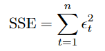
This quantity serves as the objective function to be minimized when estimating the parameters of the ARMA(p,q) model.

sse_local += errors[t] * errors[t];

ARMA(p,q) Estimation via Gradient-Based Optimization

Once the time series has been transformed into a stationary process, we can model it using an ARMA(p,q) structure.

We propose the following function:

ARMA(int p, int q, const double &Series[], double &sse, double &c, double &AR[], double &MA[])

This function takes as input the parameters p, q, and a time series. As output, it provides the estimated coefficients of the model (AR and MA components), along with the intercept c and the SSE.

To approximate the parameter values, we use c, ϕᵢ, and θⱼ from our ARMA model, and we iteratively update the coefficients using gradient-based optimization.

We begin by initializing the parameters of the ARMA model. The coefficients of the AR(p) and MA(q) components are set to zero, while the intercept c is initialized as the mean of the time series.

Then, we compute the errors of the model to evaluate its performance.

//--- Forward pass: compute predictions and errors
for(int t = 1; t < n; t++)
  {
   double pred = c;

//--- AR part
   for(int i = 0; i < p && t-1-i >= 0; i++)
      pred += AR_local[i] * Series[t-1-i];

//--- MA part
   for(int j = 0; j < q && t-1-j >= 0; j++)
     {
      pred += MA_local[j] * errors[t-1-j];
     }

   errors[t] = Series[t] - pred;
   sse_local += errors[t] * errors[t];
  }

With our stopping criteria

//--- Early stopping based on absolute SSE change
if(iter > 1 && fabs(prev_sse - sse_local) < 1e-10)
  {
   sse = sse_local;
   ArrayResize(AR, p);
   ArrayCopy(AR, AR_local);
   ArrayResize(MA, q);
   ArrayCopy(MA, MA_local);
   break;
  }

At each iteration, we compute gradients with respect to each parameter and update the coefficients to reduce the overall error.

The process stops when it reaches the maximum number of iterations or when the error change between iterations becomes negligible.

For the constant:

For the autoregressive coefficients:

For the moving average coefficients:

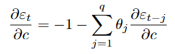
//--- Backpropagation through time (BPTT) to compute gradients
for(int t = 1; t < n; t++)
  {
//--- ∂ε_t/∂c = -1 - Σ(θ_j * ∂ε_{t-j}/∂c)
   dEdc[t] = -1.0;
   for(int j = 0; j < q && t-1-j >= 0; j++)
      dEdc[t] -= MA_local[j] * dEdc[t-1-j];

//--- ∂ε_t/∂AR_local[i]
   for(int i = 0; i < p; i++)
     {
      double der = (t-1-i >= 0) ? -Series[t-1-i] : 0.0;
      for(int j = 0; j < q && t-1-j >= 0; j++)
         der -= MA_local[j] * dEdAR[(t-1-j)*p + i];
      dEdAR[t*p + i] = der;
     }

//--- ∂ε_t/∂MA_local[j]
   for(int j = 0; j < q; j++)
     {
      double der = (t-1-j >= 0) ? -errors[t-1-j] : 0.0;
      for(int k = 0; k < q && t-1-k >= 0; k++)
         der -= MA_local[k] * dEdMA[(t-1-k)*q + j];
      dEdMA[t*q + j] = der;
     }
  }

Then we obtain the partial differentials for each of the parts of our model.

For the constant:

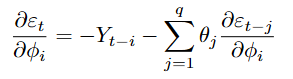
For the autoregressive coefficients:

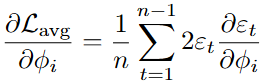
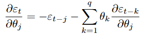
For the moving average coefficients:

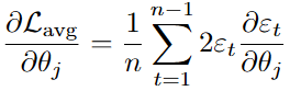
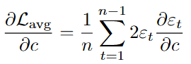
//--- Accumulate gradients of SSE with respect to parameters
double grad_c = 0.0;

for(int t = 1; t < n; t++)
  {
   grad_c += 2.0 * errors[t] * dEdc[t];
   for(int i = 0; i < p; i++)
      grad_AR[i] += 2.0 * errors[t] * dEdAR[t*p + i];
   for(int j = 0; j < q; j++)
      grad_MA[j] += 2.0 * errors[t] * dEdMA[t*q + j];
  }

//--- Average gradients over the series length
grad_c /= n;
for(int i = 0; i < p; i++)
   grad_AR[i] /= n;
for(int j = 0; j < q; j++)
   grad_MA[j] /= n;

ADAM (Adaptive Moment Estimation)

Once the average gradients of the loss function with respect to each parameter have been computed, the Adam optimizer is employed iteratively to update the parameters c, ϕᵢ, and θⱼ.

For each parameter,

The algorithm maintains two exponential moving averages based on the first and second moments of the gradients.

Let

, denote the average gradient with respect to ξ at iteration k. The biased first moment estimate

and biased second moment estimate

are updated recursively as

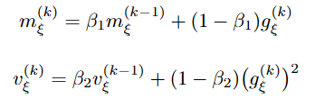
where

Since these moment estimates are initialized at zero, they are biased toward zero, particularly during early iterations. To correct this initialization bias, we compute bias-corrected estimates.

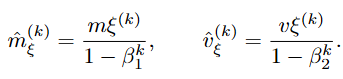
With these corrected values, the parameter ξ is updated according to the Adam rule.

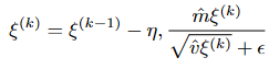
Where η > 0 is the learning rate and ϵ > 0 is a small constant added for numerical stability.

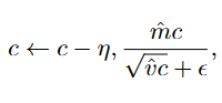
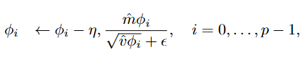
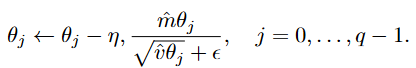
In the specific context of the ARMA model, the updates are applied individually to each parameter group:

After each update, the autoregressive and moving-average coefficients are clipped to the interval [−0.99, 0.99] to improve numerical stability and reduce the risk of non-stationary or non-invertible parameters. This helps keep the optimization stable and the resulting ARMA process well-behaved.

//--- Adam optimizer hyperparameters
double beta1 = 0.9, beta2 = 0.999, eps = 1e-8, eta   = 0.001; 

//--- Adam updates for AR coefficients
for(int i = 0; i < p; i++)
  {
   m_AR[i] = beta1 * m_AR[i] + (1-beta1) * grad_AR[i];
   v_AR[i] = beta2 * v_AR[i] + (1-beta2) * grad_AR[i] * grad_AR[i];
   double m_hat = m_AR[i] / (1 - beta1_pow);
   double v_hat = v_AR[i] / (1 - beta2_pow);
   AR_local[i] -= eta * m_hat / (sqrt(v_hat) + eps);

   //--- Clamp AR coefficients to ensure stationarity ([-0.99, 0.99])
   if(AR_local[i] > 0.99)
      AR_local[i] = 0.99;
   if(AR_local[i] < -0.99)
      AR_local[i] = -0.99;
  }

//--- Adam updates for MA coefficients
for(int j = 0; j < q; j++)
  {
   m_MA[j] = beta1 * m_MA[j] + (1-beta1) * grad_MA[j];
   v_MA[j] = beta2 * v_MA[j] + (1-beta2) * grad_MA[j] * grad_MA[j];
   double m_hat = m_MA[j] / (1 - beta1_pow);
   double v_hat = v_MA[j] / (1 - beta2_pow);
   MA_local[j] -= eta * m_hat / (sqrt(v_hat) + eps);

   //--- Clamp MA coefficients to ensure invertibility ([-0.99, 0.99])
   if(MA_local[j] > 0.99)
      MA_local[j] = 0.99;
   if(MA_local[j] < -0.99)
      MA_local[j] = -0.99;
  }

AutoARIMA

With an estimation procedure for any (p, q), we can automate model selection. First, the function differentiates the original series using the previously estimated order d. Then it performs a grid search over predefined autoregressive and moving-average orders and selects the combination with the best information-criterion value.

For each pair of p and q, we fit an ARMA(p,q) model to the differenced series using the gradient-based estimation procedure described in the previous section.

Model Evaluation

To compare models, we employ the corrected Akaike Information Criterion (AICc), which penalizes the number of parameters while adjusting for small sample sizes:

//+------------------------------------------------------------------+
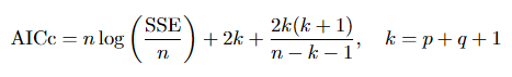
//| AICc: Akaike Information Criterion corrected                     |
//+------------------------------------------------------------------+
double AICc(const double &Series[], double sse, int p, int q)
  {
   int n = ArraySize(Series);
   int k = p + q + 1;   // Total number of parameters (AR + MA + constant)

//--- Avoid division by zero or negative degrees of freedom
   if(n - k - 1 <= 0)
      return DBL_MAX;

//--- If SSE is zero or negative, return a very large value (model invalid)
   if(sse <= 0.0)
      return DBL_MAX;

//--- Estimate residual variance
   double sigma2 = sse / n;
   if(sigma2 < 1e-15)
      return DBL_MAX;

//--- Compute standard AIC and apply finite-sample correction
   double aic  = n * MathLog(sigma2) + 2.0 * k;
   double aicc = aic + (2.0 * k * (k + 1.0)) / (double)(n - k - 1);
   return aicc;
  }

Best Model

Having defined a criterion to evaluate the quality of a fitted model, we now automate the selection of the optimal ARMA orders (p,q) for the differenced series:

//--- Define the maximum orders to test for AR and MA parts
int max_p = 5;
int max_q = 5;

//--- Variables to store the best model found
int best_p = -1, best_q = -1;
double best_c = 0.0, best_sse = DBL_MAX;
double best_AR[], best_MA[];

//--- AICc values for model comparison
double AICc_ARMA = DBL_MAX, Best_AICc = DBL_MAX;

//--- Array for the differenced (stationary) series
double diff[];

//--- Determine differencing order using a variance heuristic
int d = Calculate_d(Series);

//--- Apply d-order differencing; the result is in chronological order (oldest first)
Difference(d, Series, diff);

//--- Grid search over p and q – choose the model with the lowest AICc
for(int p=0; p<max_p; p++)
  {
   for(int q=0; q<max_q; q++)
     {
      //--- Variables passed by reference to store ARMA results
      double sse = 0.0, dummy_c;
      double dummy_AR[], dummy_MA[];

      //--- Train ARMA(p,q) on the differenced data using Adam optimizer
      ARMA(p, q, diff, sse, dummy_c, dummy_AR, dummy_MA);

      //--- Compute corrected AIC for this model
      AICc_ARMA = AICc(diff, sse, p, q);

      //--- Update best model if current AICc is lower
      if(AICc_ARMA < Best_AICc)
        {
         Best_AICc = AICc_ARMA;
         best_p = p;
         best_q = q;
         best_c = dummy_c;
         best_sse = sse;
         ArrayCopy(best_AR, dummy_AR);
         ArrayCopy(best_MA, dummy_MA);
        }
     }
  }

Forecasting

After selecting the best ARMA model, we forecast the next period. The first step is to reconstruct the error sequence for the differenced series using the optimal coefficients. We iterate through the differenced data, computing the predicted value at each time step as

//--- Recalculate the error series using the best ARMA coefficients
int n_diff = ArraySize(diff);
double errors[];
ArrayResize(errors, n_diff);
ArrayInitialize(errors, 0.0);

for(int t=1; t<n_diff; t++)
  {
   double pred = best_c;

//--- Add AR contribution
   for(int i=0; i<best_p && t-1-i>=0; i++)
      pred += best_AR[i] * diff[t-1-i];

//--- Add MA contribution (using previously computed errors)
   for(int j=0; j<best_q && t-1-j>=0; j++)
      pred += best_MA[j] * errors[t-1-j];
   errors[t] = diff[t] - pred;
  }

Next, we compute a one-step-ahead forecast for the differenced series. Using the last available index, we forecast the next difference as the sum of the constant term, the autoregressive-lag contributions, and the moving-average terms computed from the reconstructed errors.

//--- Compute one-step-ahead forecast on the differenced scale
double forecast_diff = best_c;
int last_t = n_diff-1;

for(int i=0; i<best_p; i++)
   if(last_t-i >= 0)
      forecast_diff += best_AR[i] * diff[last_t-i];

for(int j=0; j<best_q; j++)
   if(last_t-j >= 1)
      forecast_diff += best_MA[j] * errors[last_t-j];

Finally, we integrate this differenced forecast back to the original price level. The transformation depends on the differencing order d.

We then round the result to the nearest tick size.

//+------------------------------------------------------------------+
//| Round2Ticksize: rounds price to valid tick size                  |
//+------------------------------------------------------------------+
double Round2Ticksize(double price)
  {
   double tick_size = SymbolInfoDouble(_Symbol, SYMBOL_TRADE_TICK_SIZE);
   return(round(price / tick_size) * tick_size);
  }

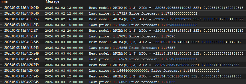
The function returns the final price forecast and prints the best model diagnostics.

forecast_price = Round2Ticksize(forecast_price);

Print("Best model: ARIMA(", best_p, ",", d, ",", best_q, ") AICc = ", Best_AICc, " SSE: ", best_sse);
Print("Last price: ", Series[0], " Price forecast: ", forecast_price);
return forecast_price;

Usage of AutoARIMA

The AutoARIMA() function is called on a price series and returns a one-step-ahead forecast. It requires minimal configuration.

The function expects a single array containing the most recent prices of the financial instrument, ordered from the most recent to the oldest value.

AutoARIMA(Close)

Then it returns a double value representing the forecasted price for the next time period.

double forecast = AutoARIMA(Close);

Function in action

To illustrate the behavior of the AutoARIMA implementation, we execute the function on the Nikkei 225 index using a four‑hour (H4) timeframe. The input series is constructed from the most recent closing prices, with the latest value stored at index 0.

//+------------------------------------------------------------------+
//| Expert tick function                                             |
//+------------------------------------------------------------------+
void OnTick()
  {
//--- Detect new bar formation
   bool isNewBar = false;
   int CurrBar = iBars(_Symbol, PERIOD_CURRENT);   // total bars on chart now
   static int PrevBar = CurrBar;                   // remember previous count

   if(PrevBar == CurrBar)
      isNewBar = false;                            // no new bar yet
   else
     {
      isNewBar = true;                             // a new bar has appeared
      PrevBar = CurrBar;                           // update the reference count
     }

//--- When a new bar completes, run the ARIMA model
   if(isNewBar)
     {
      int Candles_To_Copy = 5000;                  // lookback size for training

      double Close[];
      ArrayResize(Close, Candles_To_Copy);
      CopyClose(Symbol(), PERIOD_CURRENT, 0, Candles_To_Copy, Close);
      ArraySetAsSeries(Close, true);               // index 0 = most recent price

      double forecast = AutoARIMA(Close);          // forecast for the next bar
     }
  }

Conclusion

The article delivers an executable AutoARIMA module for MQL5 with a clear contract: AutoARIMA(Close[]) takes an array of recent closing ordered prices from newest to oldest and returns a double—the one-step-ahead price forecast—while printing diagnostics (Best model: ARIMA(p,d,q), AICc, SSE, last price, forecast). The implementation fixes the main engineering decisions needed to make ARIMA practical in a trading environment: a variance-based d estimator, SSE as the objective, gradient calculations for parameter sensitivities, Adam for stable iterative updates, and clipping of AR/MA coefficients to [−0.99, 0.99] to avoid non-stationary/invertible solutions. Model selection is automated by grid search over (p,q) with AICc penalization, and the forecast is converted back to price-space and rounded to the instrument tick.

imitations and practical notes: the routine produces a single-step forecast only; d is a heuristic (not a formal unit-root test); the grid search uses bounded orders (defaults like max p = max q = 5) to keep runtime acceptable; and reliable results require a sufficient history of observations. Use AutoARIMA(Close) as a plug-in predictive feature—a signal filter, target level, or input to higher-level decision logic—and consider extensions (ADF-based d-selection, wider p/q grid, multi-step forecasting, or alternative estimators) if you need stronger statistical guarantees or multi-horizon forecasts.