Neural Networks in Trading: Effective Feature Extraction for Accurate Classification (Mantis)

Introduction

In a world where milliseconds and the slightest price fluctuations are critical, traders seek tools that can not only predict future price movements but also accurately classify the most complex patterns on charts. In this context, the Mantis foundation model, proposed in the article “Mantis: Lightweight Calibrated Foundation Model for User-Friendly Time Series Classification,” opens a new chapter in time series analysis. With its lightweight design, well-thought-out architecture, and excellent calibration, Mantis makes it possible to quickly integrate the classifier into trading systems and obtain reliable confidence estimates for risk management.

The authors note that traditional approaches trained to predict subsequent values often prove too sluggish: they require careful fine-tuning for each new strategy, and large volatility spikes can significantly impair their performance. That said, in recent years, foundation models for time series forecasting have delivered impressive results, but they are essentially designed for regression rather than for classifying market regimes. This is precisely the gap the authors filled by introducing the Mantis framework with contrastive pre-training.

The idea is simple and elegant: split the time series into a series of patches and then, much like the Vision Transformer in computer vision, apply hybrid attention. However, the classic global attention mechanism has quadratic complexity, which becomes a bottleneck for high-frequency data. To mitigate this effect, Mantis simultaneously uses local tokens—obtained through convolutions and pooling over small windows — and global tokens, which aggregate trend information over the entire segment. This combination provides nearly linear scalability with respect to the series length and preserves the ability to capture both small fluctuations and long-term patterns.

Contrastive pre-training in Mantis is the secret sauce that pulls together different augmentations of the same time segment while pushing radically different time series apart. As a result, embeddings of the same pattern with different variations cluster together in space, while different events move apart. This strategy allows the model to learn stable features of various patterns, even though the peaks and troughs may shift in amplitude and time.

A key aspect for a trader is assessing whether it is safe to open a position: it is not enough to simply say, “This is a trend reversal”; one needs to understand how confident the model is in its conclusion. Mantis solves this problem with a built-in temperature scaling module: it adjusts the output logits so that the posterior probabilities better reflect the empirical likelihood of belonging to a class. As a result, when a signal is labeled “80% probability of a reversal,” a trader can expect that the signal will be correct in about four out of five cases.

The authors also paid particular attention to multivariate analysis: algorithmic trading often involves the simultaneous use of dozens of indicators (moving averages, RSI, trading volumes, currency pair correlations, etc.). Simply combining all channels into a single high-dimensional representation leads to an explosion in the number of parameters and increased memory requirements, while analyzing univariate sequences strips away information about inter-channel dependencies. Therefore, the framework's developers have built in lightweight adapters that condense cross-channel interactions into a compact space without losing information about the relationships between different indicators.

To illustrate the practical value of Mantis, imagine a “flash crash” scenario in the cryptocurrency market: within a second, the price plummets by several percent and then rebounds just as rapidly. A classical model might interpret this anomaly as noise and ignore the entry signal. Mantis, thanks to pre-training on millions of real and synthetic examples, understands that such events can be either “false” or “true”: it assigns a label of “short-term anomaly” or “genuine reversal” with different confidence estimates, allowing the trader to develop an appropriate capital preservation strategy.

Another real-world example is the classification of market regimes for technology stocks. During an uptrend, prices move almost in sync due to the overall news backdrop, while during a correction, each asset behaves in its own way. Mantis, thanks to its adapters, detects these cross-channel discrepancies: low correlation between similar assets becomes a signal of the start of a correction cycle, which the model reports along with a confidence estimate.

Mantis Algorithm

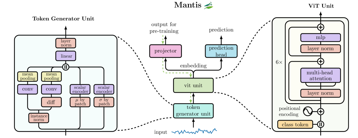
The Mantis framework demonstrates how well-thought-out architecture and thorough training can transform a set of ideas into a reliable tool. The foundation-model approach presented by the authors of the framework rests on four key pillars: time series tokenization, hybrid attention, adapters for multivariate data, and Self-Supervised contrastive pre-training followed by calibration.

The main idea behind Mantis is to move away from the traditional practice of dividing a time series into fixed windows. Instead, the sequence is divided into a fixed number of patches, which ensures independence from the length of the input sequence and stabilizes the computational cost. For example, series of lengths 1024 and 2048 will be converted into the same number of patches — 32. This approach is critically important for large-scale processing of heterogeneous time series.

The embedding is formed in several stages. First, a convolutional layer with 256 output channels is applied. This layer transforms the time series into a more compact latent representation. Next, each of the 32 patches is aggregated using averaging (mean pooling), resulting in a tensor of dimension (32, 256). Each patch encodes the local characteristics of the time series, including peaks, fluctuations, and the microstructure of price movements.

In parallel, a second data stream — the differential stream — is created. It is based on the first differences between adjacent values in the time series. This transformation helps eliminate long-term trends and amplify signals related to short-term dynamics. It is particularly useful in situations where deviations from a stable level or sharp movements near support and resistance levels are of interest.

Both streams undergo the same processing steps: convolution, averaging, and normalization. The result is two sets of patches, each containing 32 tokens of dimension 256. This provides the model with balanced information about both the signal's shape and its changes over time.

In addition, two more types of information are extracted: scale and volatility. To do this, the time series is divided into 32 equal windows, and the mean and standard deviation are calculated for each window. These statistics are encoded using the Multi-Scaled Scalar Encoder, which allows the model to capture the background characteristics of the signal. Thus, the model receives four data streams at once: normalized values, differentials, mean values, and standard deviations.

The four data streams are combined by concatenation. Before that, they are passed through individual linear projectors to ensure dimensional consistency. Next, the combined embeddings pass through a projection layer followed by Layer Normalization, resulting in a final representation of the time series as 32 tokens of dimension 256. These tokens are universal containers that hold behavioral and statistical information about the market.

The next step in the architecture is to add a class token — a trainable vector whose task is to aggregate information from all tokens. This allows the model to form the final representation of the series, taking into account both local and global patterns. To preserve information about the order of the patches, sinusoidal positional encoding is applied, after which the data is fed into the Transformer block.

The Transformer consists of six layers. Each layer contains an 8-head Multi-Head Attention mechanism, a normalization layer, and a two-layer feed-forward block with GELU activation. During the pre-training phase, dropout is applied with a probability of 10%, which helps prevent overfitting. After all layers have been passed through, the class-token output vector is used to form the final sequence embedding.

Mantis is trained using a self-supervised paradigm that incorporates contrastive learning. The model applies a variety of time-series augmentations to the source data. Specifically, in the RandomCropResize method, 0 to 20% of the sequence is randomly removed, and the remaining portion is stretched back to the original length. This preserves the overall structure of the signal without altering the sequence of events.

For each example xi in the batch, two augmentations are randomly selected. The resulting representations are passed through a projection head and compared using cosine similarity.

Then the cross-entropy loss is computed.

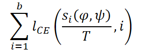
In their work, the framework’s authors pre-trained the model on a combined sample from 10 datasets, comprising more than 7 million time series. Training ran for 100 epochs. A batch size of 2048 was used, along with four Tesla V100-32GB GPUs.

During fine-tuning, a classification head was attached to the embedding. The resulting forecast values undergo temperature scaling, which minimizes the expected calibration error and allows the model’s results to be interpreted in probabilistic terms.

However, the multivariate nature of time series remains one of the main challenges. Different tasks may involve different numbers of channels, which requires adapting the model. Like other foundation models, Mantis is trained in a univariate form and applies the same mechanism to each channel. This not only increases the burden on computational resources, but also ignores cross-channel correlations.

To address these limitations, the framework’s authors propose using a channel adapter — a function a that transforms the original d channels into dnew. This approach makes it possible to adapt the input data to the computational budget, preserve the temporal structure, and ensure compatibility with any model.

Here, the authors of the Mantis framework consider five adapter variants. The first four are classic dimensionality reduction methods:

• PCA (Principal Component Analysis): finds an orthogonal space in which most of the variance is concentrated in a smaller number of components;
• Truncated SVD: similar to PCA, but applied to the uncentered data matrix;
• Random Projection: a random linear mapping to a lower-dimensional space;
• Variance-Based Selector: selects the channels with the highest variance.

The data for these adapters is reshaped to the form (n*t, d), where n is the number of examples. The projection matrix W performs the channel mapping.

The fifth adapter — Differentiable Linear Combiner (LComb) — is trained alongside the main model by adjusting its parameters during the backward pass. This makes it possible to take the context of the task into account and achieve greater accuracy.

As a result, Mantis is suitable for a wide range of tasks without losing the temporal structure of the data or the inter-channel relationships. The model remains versatile and efficient, even in real-world multivariate scenarios.

The authors' visualization of the Mantis framework is shown below.

Implementation Using MQL5

After a thorough analysis of the theoretical aspects of the Mantis framework, it is time to move on to the most interesting part — its practical implementation. This is where the ideas take concrete form in code, that ideas take shape and abstract principles begin to yield results. Our focus is on the software implementation of the framework’s key architectural decisions using the MQL5 language. Despite the high complexity of the concepts, we face a clear and ambitious challenge: to build a model capable of effectively processing real-world market data, adapting to volatility, and at the same time remaining as resource-efficient as possible.

Discussion of Approaches

Before we start writing code, as is standard practice in engineering, we need to develop a strategy. Without a clear plan, no architecture can withstand the demands of real-world markets. Our journey begins with a systematic analysis: what exactly we want to implement, what roles the individual components play, and where potential bottlenecks may be hidden. It is important not just to copy the authors' ideas, but to adapt them to our task and the MQL5 environment, which has its own limitations and unique features.

At the heart of the implementation is token formation. This is where the foundations of the model's future success are laid, since Transformer cannot process raw data effectively. It requires input in the form of token sequences, each of which carries a compressed yet expressive representation of a portion of the time series.

The original Mantis architecture proposes using a multichannel scheme that includes deviation series, segment means, and segment standard deviations. However, with normalized inputs, which our models most often work with, the information value of the mean-value and standard-deviation streams decreases. We deliberately discard these channels, focusing instead on two key streams: the original time series and its first difference. This combination makes it possible to account for both global levels and local changes at the same time — a kind of compromise between stability and sensitivity.

The process of preparing these streams begins with normalizing the original time series. This is an important step that helps smooth out large-scale fluctuations and improve the model's resilience to outliers. Next, a differencing operation is applied to calculate the difference between adjacent observations. The resulting series is highly responsive to sudden changes, which is particularly valuable when trying to capture market impulses or reversals. After that, the two series are combined into a two-channel tensor, where each channel represents a separate information stream.

However, simply combining them is not enough. Despite the wealth of information contained in a multichannel time series, the model still lacks crucial information about temporal context. As is well known, transformers do not have a built-in ability to understand the order of elements in the input sequence; therefore, they require additional information describing the position of each observation relative to the others.

In the original Mantis implementation, this problem was solved by adding sinusoidal positional encoding similar to that proposed in Attention Is All You Need. This approach is convenient because of its versatility and portability: it requires no training and works well on tasks of various kinds. At the same time, the encoding is added only after the channels have been combined and segmented into patches.

However, we propose a different approach. Before splitting the sequence into fragments, we introduce temporal encoding, similar to the Mamba4Cast framework. This encoding not only indicates a point’s position on the time grid, but also conveys information about the temporal structure of the time series — it allows the model to detect hidden seasonality, recurring patterns, asymmetries, and rhythms in market data. Unlike sinusoidal encoding, temporal encoding is more sensitive to the market's microstructure and can capture patterns that extend beyond the current analysis window.

Only after adding this encoding can we move on to the next logical step — channel segmentation. This step acts as a kind of filter that transforms temporally enriched information into a form suitable for the model. In other words, by this point, the data already carry not only the value and the derivative, but also an additional layer of context that reveals their behavioral dynamics over time. This significantly simplifies the model's task of identifying complex relationships and makes its performance more resilient to market noise.

I suggest we discuss the changes to the segmentation algorithm a little later, when we get to the actual implementation. For now, we are deliberately setting aside descriptions of the other modules in order to focus on the foundation — the transformation of a time series into an informative, standardized, and structured sequence. It is at this stage that the success of the entire model is laid. Well-prepared data make it possible to effectively identify patterns, correctly account for the order of events, and distinguish important patterns in market behavior.

Now that the conceptual framework is in place and the roadmap has been outlined, it is time to move from words to action. At this stage, the actual implementation of the model begins — the very moment when theory is transformed into lines of code. Let's start with the most basic — and yet extremely important — part: the preprocessing of the time series, which results in a multichannel representation of the data. This is where the initial feature extraction takes place, which will subsequently determine what Transformer sees and how it interprets it. The task is to extract two streams: the original series and its first difference, and then combine them into a single tensor. We implement all of this using OpenCL.

Changes to the OpenCL Program

The use of OpenCL is driven by the need to accelerate computations, especially when working with a large number of time series. The GPU makes it possible to parallelize operations over multiple variables and speed up data preparation without burdening the main processor. Therefore, the first thing we will implement is a specialized ConcatDiff kernel. Its purpose is to compute the first difference and concatenate the result with the original data at the same time, thereby forming a tensor with two channels for each time interval.

Only two pointers to data buffers are passed as parameters to this kernel — a time-tested minimalist approach. The first is the input array data, which contains the time series being analyzed, and the second is the output buffer output, where the calculation results are stored. This approach makes the kernel interface as simple and intuitive as possible, eliminating unnecessary overhead.

The additional parameter is the constant step — the step size used to calculate the difference. This addition makes the algorithm significantly more flexible. Now we can calculate both the classic first difference (between adjacent points) and, for example, the difference between the value "now" and the value "five steps ahead." The latter can be particularly useful in a financial context: this parameter makes it possible to prepare features that reflect changes across different time horizons.

__kernel void ConcatDiff(__global const float* data,
                         __global float* output,
                         const int step)
  {
   const size_t i = get_global_id(0);
   const size_t v = get_local_id(1);
   const size_t inputs = get_local_size(0);
   const size_t variables = get_local_size(1);

Each work-item is assigned a unique pair of indices — a time index i and a variable index v. Thus, each work-item is responsible for processing a single specific value in the source data matrix.

The source data array data is a normalized time series represented in linearized form, with time and channel dimensions unfolded.

Next, inside the kernel, we compute shift — the offset in the data array corresponding to the current time-channel position.

const int shift = i * variables;
const float d = data[shift + v];

After obtaining the original value d, we proceed to compute its first difference along the time axis. To do this, we take the difference between the current value and the value located step steps ahead. This approach is intended for preparing features that reflect local dynamics: growth or decline, acceleration or deceleration of change. In doing so, the index must be checked for validity: we must not go beyond the bounds of the array.

float diff = 0;
if(step > 0 && (i + step) < inputs)
   diff = IsNaNOrInf(d - data[shift + step * variables + v], 0);

The difference computation ends with the protective function IsNaNOrInf, which sets the result to zero if NaN or infinity appears — this is especially important when missing values or data glitches are present.

Next comes the key stage — forming the output array output. An interesting operation takes place here: the data are written in pairs. First, the original value is recorded, followed by the corresponding value of the first difference. Since we use a doubled variable stride (twice as many channels), the resulting tensor for each time step contains two values for each variable. Thus, the output structure has a size of (T * 2 * V), where T is the number of time steps and V is the number of variables.

 output[2 * shift + v] = d;
 output[2 * shift + v + variables] = diff;
}

This approach allows the data to be prepared for feeding into the model in a single pass: the tensor already contains both static and dynamic market characteristics.

Using OpenCL in this case offers a twofold benefit: it saves time (through parallel processing) and simplifies the code logic, since all operations involving indices and arrays are performed within the kernel. Instead of cumbersome loops on the CPU side, we have a compact and efficient block that can be easily scaled to handle data of any length and width.

This module serves as the first building block in the foundation of the entire model. It implements a key concept: the initial decomposition of a time series into two complementary streams. The original values make it possible to see levels and trends, while the first difference provides sensitivity to changes — a kind of derivative that signals turning points. Together, they create a balanced representation that is robust to noise and adaptive to rapid changes.

It is worth emphasizing an architectural feature of this stage: the ConcatDiff kernel contains no trainable parameters. Its purpose is purely functional — to perform simple linear operations (extracting values and computing their differences) and combine the results into a single array. All of this makes it exceptionally well suited for implementation in OpenCL, where massively parallel processing operations without complex state logic are particularly effective.

Moreover, given the specific nature of financial time series, it is entirely logical to treat the input data themselves as constant within a single preparation iteration. That is precisely why, in this case, we do not implement kernels for backpropagation of the error gradient or for updating parameters. Such tasks are relevant only to the trainable layers that make up the model. Here, however, we are dealing with preprocessing — a stage where speed, reliability, and fully deterministic computations are crucial.

The complete code for the OpenCL program is provided in the attachment.

Difference calculation object

The next step in our work is to integrate the ConcatDiff kernel into the main program's structure. To do this, we create a specialized object implemented as the CNeuronConcatDiff class. This object serves as an interface between the logic of the high-level neural network model and the low-level OpenCL code, ensuring that parameters are properly prepared, the kernel is launched, and the result is received.

class CNeuronConcatDiff:  public CNeuronBaseOCL
  {
protected:
   uint              iUnits;
   uint              iVariables;
   uint              iStep;
   //---
   virtual bool      feedForward(CNeuronBaseOCL *NeuronOCL) override;
   virtual bool      updateInputWeights(CNeuronBaseOCL *NeuronOCL) override   { return true; }
   virtual bool      calcInputGradients(CNeuronBaseOCL *NeuronOCL) override;

public:
                     CNeuronConcatDiff(void) :  iUnits(0), iVariables(1), iStep(1) {  activation = None; }
                    ~CNeuronConcatDiff(void) {};
   virtual bool      Init(uint numOutputs, uint myIndex, COpenCLMy *open_cl,
                          uint units_count, uint step, uint variables,
                          ENUM_OPTIMIZATION optimization_type, uint batch);
   //---
   virtual int       Type(void) override  const   {  return defNeuronConcatDiff;   }
   //--- methods for working with files
   virtual bool      Save(int const file_handle) override;
   virtual bool      Load(int const file_handle) override;
  };

The class itself includes several key variables:

• iUnits — the number of time steps,
• iVariables — the number of channels or variables in the source data,
• iStep — a shift parameter that specifies the step size for calculating the difference. This value makes the component versatile — it can be adapted to any time-window width or sampling rate.

The class constructor initializes the key parameters with default values: one channel (iVariables = 1), a step size of one (iStep = 1), and the activation function disabled (activation = None), which makes sense — after all, our component operates at the preprocessing stage and should not introduce nonlinearities.

The class also implements an object initialization method called Init, whose parameters receive constants that make it possible to unambiguously interpret the architecture of the object being created.

bool CNeuronConcatDiff::Init(uint numOutputs, uint myIndex, COpenCLMy *open_cl,
                             uint units_count, uint step, uint variables,
                             ENUM_OPTIMIZATION optimization_type, uint batch)
  {
   if(!CNeuronBaseOCL::Init(numOutputs, myIndex, open_cl, 2 * units_count * variables, optimization_type, batch))
      return false;
   if(step<=0 || step >= units_count)
      return false;
//---
   iUnits = units_count;
   iVariables = variables;
   iStep = step;
//---
   return true;
  }

The logic behind the Init method is as simple and concise as possible. In its body, the parent class function of the same name is called, taking into account the specifics of the data structure. Since we combine the input data and the first difference values into the output array, the size of the output buffer must be doubled.

After the parent part is initialized, all parameters received as input are stored in the class internal variables. This allows them to be used when forming the parameters for the OpenCL kernel.

This approach makes the object flexible, independent, and reusable.

Special attention is given to the virtual feedForward method, which is responsible for the forward pass and, consequently, for calling the OpenCL kernel.

In the method parameters, we receive a pointer to the source data object and immediately verify its validity.

bool CNeuronConcatDiff::feedForward(CNeuronBaseOCL *NeuronOCL)
  {
   if(!OpenCL || !NeuronOCL || !Output)
      return false;
   if(getOutputIndex() < 0)
      return false;

After successfully passing the set of checks, the ConcatDiff kernel is queued for execution. This uses the algorithm you are already familiar with. The values previously stored in internal variables are used to specify the dimensionality of the task space.

{
 uint global_work_offset[2] = {0};
 uint global_work_size[2] = {iUnits, iVariables};
 const int kernel = def_k_ConcatDiff;
 if(!OpenCL.SetArgumentBuffer(kernel, def_k_concdiff_data, NeuronOCL.getOutputIndex()))
   {
    printf("Error of set parameter kernel %s: %d; line %d", OpenCL.GetKernelName(kernel),
                                                               GetLastError(), __LINE__);
    return false;
   }
 if(!OpenCL.SetArgumentBuffer(kernel, def_k_concdiff_output, getOutputIndex()))
   {
    printf("Error of set parameter kernel %s: %d; line %d", OpenCL.GetKernelName(kernel), 
                                                               GetLastError(), __LINE__);
    return false;
   }
 if(!OpenCL.SetArgument(kernel, def_k_concdiff_step, iStep))
   {
    printf("Error of set parameter kernel %s: %d; line %d", OpenCL.GetKernelName(kernel), 
                                                               GetLastError(), __LINE__);
    return false;
   }
 //---
 if(!OpenCL.Execute(kernel, global_work_size.Size(), global_work_offset, global_work_size))
   {
    printf("Error of set parameter kernel %s: %d; line %d", OpenCL.GetKernelName(kernel), 
                                                               GetLastError(), __LINE__);
    return false;
   }
}

However, the feedForward method does not end there. The next step is to normalize the resulting tensor — essentially, bringing the data to a uniform scale, which is critically important when training a neural network. Moreover, this implementation performs separate normalization for features (the original values of the variables are normalized) and for differences (the first difference values are processed separately). This allows the model to remain sensitive to sharp changes in the time series without losing its stability in the face of large-scale fluctuations.

     {
      uint global_work_offset[1] = {0};
      uint global_work_size[1] = {2 * iUnits};
      const int kernel = def_k_Normilize;
      if(!OpenCL.SetArgumentBuffer(kernel, def_k_norm_buffer, getOutputIndex()))
        {
         printf("Error of set parameter kernel %s: %d; line %d", OpenCL.GetKernelName(kernel),
                                                                    GetLastError(), __LINE__);
         return false;
        }
      if(!OpenCL.SetArgument(kernel, def_k_norm_dimension, iVariables))
        {
         printf("Error of set parameter kernel %s: %d; line %d", OpenCL.GetKernelName(kernel), 
                                                                    GetLastError(), __LINE__);
         return false;
        }
      if(!OpenCL.Execute(kernel, global_work_size.Size(), global_work_offset, global_work_size))
        {
         string error;
         CLGetInfoString(OpenCL.GetContext(), CL_ERROR_DESCRIPTION, error);
         printf("Error of execution kernel %s: %d -> %s", OpenCL.GetKernelName(kernel), 
                                                                GetLastError(), error);
         return false;
        }
     }
//---
   return true;
  }

This type of post-processing significantly improves training stability and accelerates model convergence by standardizing the range of input values.

It is also worth saying a few words about the error gradient propagation method — calcInputGradients. Although we do not create a backward pass kernel for this layer, the corresponding method is still implemented.

Why? The answer is simple. This allows us to embed this object at any level of the model without worrying about breaking the error backpropagation chain. Even if this layer does not need to compute its own gradients, it must correctly pass the error signal on to the preceding objects. Otherwise, training of the entire model may fail at this layer, which will lead to stagnation of the gradient flow and, as a result, make it impossible to optimize the parameters of the lower layers.

The algorithm behind the method is simple and reliable. We obtain a pointer to the source data object (NeuronOCL) and immediately check its validity.

bool CNeuronConcatDiff::calcInputGradients(CNeuronBaseOCL *NeuronOCL)
  {
   if(!NeuronOCL)
      return false;

We redirect the error gradient accumulated in the current object along the forward information flow of the source data, using it as a signal for the previous layer. This process is pure deconcatenation without any computational tricks.

if(!DeConcat(NeuronOCL.getGradient(), getPrevOutput(), getGradient(), iVariables, iVariables, iUnits))
   return false;

If necessary (depending on the architecture), the error gradient can be adjusted using the derivative of the activation function.

   if(NeuronOCL.Activation() != None)
      if(!DeActivation(NeuronOCL.getOutput(), NeuronOCL.getGradient(), NeuronOCL.getGradient(),
                                                                       NeuronOCL.Activation()))
         return false;
//---
   return true;
  }

This approach ensures the compatibility and flexibility of the architecture. The CNeuronConcatDiff object does not interfere with gradient propagation and can be used within complex models — both at lower levels (near the input) and deep within the computational graph.

This concludes our discussion of the algorithms used to implement the methods of the CNeuronConcatDiff class. The complete code for this class and all of its methods can be found in the attachment.

We have gradually reached the limits of what is a reasonable length for this article. Despite this, the bulk of the work is still ahead of us. We have only laid the foundation. However, that is not the end of the story. To avoid overwhelming the reader and to keep the article easy to read, let’s take a short break and continue with the implementation in the next article in this series. An equally interesting and technically rich stage awaits us there.

Conclusion

In this article, we explored the Mantis framework, which combines lightweight design with high accuracy. The framework’s authors proposed an innovative approach to tokenization based on convolution and mean-pooling, which allows time series to be efficiently represented as 32 tokens of dimension 256, reducing computational costs compared to traditional methods. Contrastive pre-training on examples from diverse datasets produced a robust and transferable feature representation, outperforming other approaches in zero-shot and fine-tuning settings and achieving a record-low calibration error.

The practical section presents an implementation of the key data preprocessing layer using OpenCL and MQL5, ensuring parallel and deterministic preparation of the input tensors. In the next article, we will continue implementing our own vision of the approaches proposed by the authors of the Mantis framework.

Links

• Mantis: Lightweight Calibrated Foundation Model for User-Friendly Time Series Classification
• Other articles in this series

Software used in the article

#	Name	Type	Description
1	Research.mq5	Expert Advisor	Expert Advisor for collecting examples
2	ResearchRealORL.mq5	Expert Advisor	Expert Advisor for collecting examples using the Real-ORL method
3	StudyContrast.mq5	Expert Advisor	Expert Advisor for encoder contrastive learning
4	Study.mq5	Expert Advisor	Expert Advisor for offline model training
5	StudyOnline.mq5	Expert Advisor	Expert Advisor for online model training
6	Test.mq5	Expert Advisor	Expert Advisor for model testing
7	Trajectory.mqh	Class Library	Structure for describing the system state and model architecture
8	NeuroNet.mqh	Class Library	A class library for building neural networks
9	NeuroNet.cl	Library	Code library for the OpenCL program