

From One Price to Four: Range-Based Volatility Estimators for MetaTrader 5
 1 175
1 175
 0
0

Contents
- Introduction
- Why close-to-close throws away three quarters of every bar
- The four estimators, from naive to gap-robust
- Building the library: CVolatilityEstimators
- Indicator 1: seeing the efficiency difference
- Indicator 2: gap-aware volatility bands
- Edge cases and pitfalls
- Using the library in your own code
- Conclusion
Introduction
Almost every volatility tool a MetaTrader 5 user reaches for is built on one value per bar. Bollinger Bands take the standard deviation of closing prices. The Average True Range is closer in spirit to what we want, but it is a smoothing of a range, not a variance estimate, and it is rarely treated as one. Meanwhile every bar the terminal draws contains four prices: open, high, low, and close, and the intrabar high and low carry a great deal of information about how much the price actually moved. Discarding them is a measurable waste.
The academic literature settled this question decades ago. A family of range-based estimators, beginning with Parkinson in 1980 and refined by Garman and Klass the same year, then by Rogers and Satchell, and finally by Yang and Zhang in 2000, extracts far more information from the same bars. For a given window length, a good range estimator reaches the same statistical precision as close-to-close using a fraction of the data, or equivalently, it produces a far smoother, more responsive volatility series from the window you already have. Yet MetaTrader 5 does not provide them as standard indicators, and the CodeBase lacks a clean, reusable implementation of this classic family: a search turns up GARCH models and basic ATR, but nothing that packages Parkinson, Garman-Klass and Yang-Zhang behind one interface.
In this article we close that gap. We build a single, self-contained library, VolatilityEstimators.mqh, implementing four estimators, from the naive baseline to the most sophisticated. We then use it to build two indicators. The first is a comparison panel that plots all four together, so you can see the efficiency difference on your own charts. The second is a practical tool: volatility bands sized by the gap-robust Yang-Zhang estimator instead of a standard deviation of closes. By the end you will understand what each estimator measures, why they differ, when each one is the right choice, and you will have working code you can drop into your own projects.
You do not need any external libraries or tick data. Everything here works on standard OHLC bars, and the whole thing compiles in MetaEditor with no dependencies beyond the platform.
The short version, if you only want one default. Use Yang-Zhang on anything with real session breaks (stocks, indices, futures, and forex across the weekend), because it is the only one of the four that measures the overnight gap directly. On a near-continuous market it barely differs from the cheaper Garman-Klass. The rest of the article explains why, and provides all four through a single interface, so you can switch with one input.
Why close-to-close throws away three quarters of every bar
The standard measure of historical volatility is the sample standard deviation of logarithmic returns. For a series of closing prices, we form the log return of each bar relative to the previous one, then take the standard deviation of those returns over a window:
r_t = ln(C_t / C_{t-1})
sigma^2 = (1/(N-1)) * sum_{t=1..N} (r_t - r_bar)^2
This is correct, unbiased, and wasteful. It looks only at closing prices. If a bar opened at 1.1000, spiked to 1.1080, fell to 1.0950, and closed back at 1.1005, the close-to-close estimator sees a move of five pips. The bar actually traversed 130 pips of range. Every one of those excursions is real volatility, and the estimator is blind to all of it.
The consequence is statistical inefficiency. The variance of the close-to-close estimator itself, that is, how much its output jumps around from window to window purely because of sampling noise, is large. To get a stable reading you need a long window, and a long window lags. Range-based estimators attack this directly: by using the high and the low, they see the intrabar path and estimate the same underlying volatility with much less noise. Parkinson's estimator is roughly five times more efficient than close-to-close, Garman-Klass around seven to eight times. That efficiency is not a marginal improvement, it is the difference between a usable reading at a 20-bar window and needing a hundred bars for the same stability.
A note on the word "efficiency." Throughout this article, efficiency has its precise statistical meaning: the ratio of the variances of two estimators of the same quantity. An estimator that is "five times more efficient" produces the same estimator variance from one fifth of the data. It does not mean the code runs faster.
The catch is that every gain comes with an assumption, and the estimators differ mainly in which assumptions they make. That is the subject of the next section, and it is the key to choosing the right one.
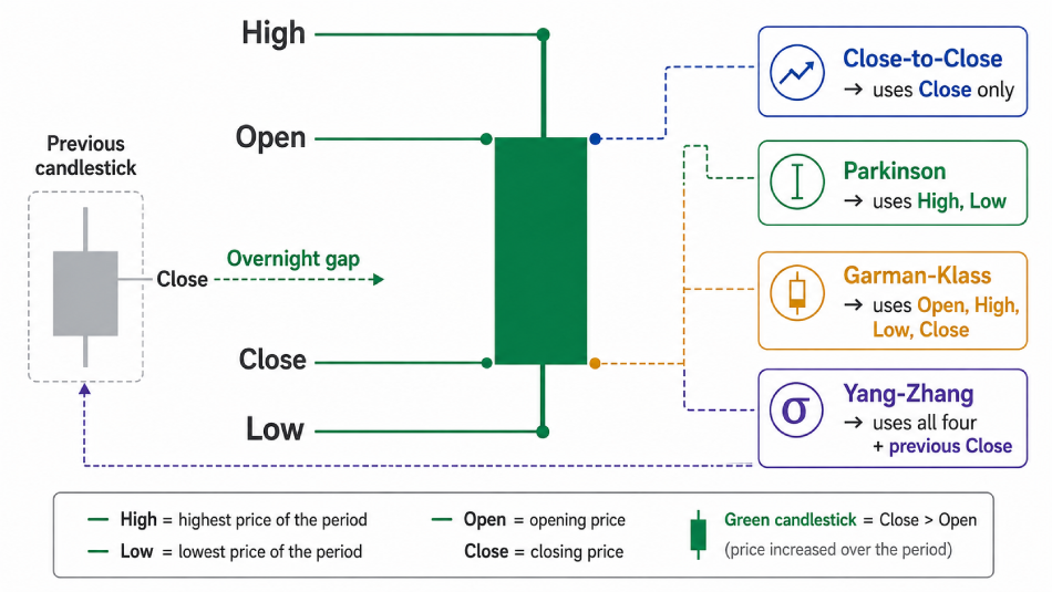
Fig. 1. One candle's four prices plus the previous close. Each estimator uses a different subset.
The four estimators, from naive to gap-robust
We implement four estimators. Presented in order, they tell a story: each one relaxes an unrealistic assumption of the one before it, at the cost of a little more machinery. Understanding that progression is more useful than memorizing the formulas, because it tells you which estimator matches your instrument and timeframe.
1. Close-to-Close, the baseline. Already covered above. Uses only closes. Makes no assumption about intrabar behavior because it ignores intrabar behavior entirely. It is the honest baseline against which we measure the others.
2. Parkinson (1980), the high-low range. Parkinson's insight was that under a driftless geometric Brownian motion, the expected squared log-range of a bar is proportional to its variance. So the range itself is an estimator:
sigma^2 = (1/(4 N ln2)) * sum_{t=1..N} ln^2(H_t / L_t)
The 1/(4 ln2) factor is the constant that makes the expected squared range equal the variance. Parkinson is far more efficient than close-to-close, but it buys that efficiency with two assumptions: the price follows a continuous path with no drift, and there are no jumps between bars. Because it never looks at the open or the previous close, it cannot see an overnight gap at all. On a market that gaps, Parkinson systematically understates volatility, because the gap moved the price but left no trace inside any single bar's high-low range.
3. Garman-Klass (1980), the full bar. Garman and Klass extended the idea to use the whole bar, combining the high-low range with the open-to-close move to squeeze out more efficiency still:
sigma^2 = (1/N) * sum_{t=1..N} [ 0.5 * ln^2(H_t / L_t) - (2 ln2 - 1) * ln^2(C_t / O_t) ]
This is the most efficient of the estimators under ideal conditions. But notice what it still does not contain: the previous close. Garman-Klass treats each bar's open as continuous with the prior close, so like Parkinson it is blind to overnight gaps and shares its downward bias on anything that gaps.
4. Yang-Zhang (2000), drift- and gap-independent. Yang and Zhang built the estimator that fixes both problems at once. It is the sum of three components: the variance of the overnight return, the variance of the open-to-close return, and the Rogers-Satchell term, which is itself a clever intrabar estimator that remains unbiased in the presence of drift.
sigma^2 = sigma_overnight^2 + k * sigma_open-close^2 + (1 - k) * sigma_RS^2
The overnight component is the variance of the overnight return, the open-to-close component the variance of the open-to-close return, and the Rogers-Satchell term is a mean of intrabar products, defined as follows:
o_t = ln(O_t / C_{t-1})                                    // overnight return
u_t = ln(C_t / O_t)                                        // open-to-close return
RS_t = ln(H_t/C_t)*ln(H_t/O_t) + ln(L_t/C_t)*ln(L_t/O_t)   // Rogers-Satchell term
k = 0.34 / (1.34 + (N+1)/(N-1))                            // blend weight
The point of all this structure: the overnight term measures close-to-open (overnight) moves directly, so Yang-Zhang reacts to the gaps that Parkinson and Garman-Klass miss, while the Rogers-Satchell component keeps it unbiased under drift. It pays for that robustness with slightly lower peak efficiency than Garman-Klass on near-continuous data, almost always a trade worth making on real markets. This is the estimator the bands indicator will use.
The table below summarizes what each estimator uses and assumes. This is the decision guide: match the row to your instrument.
| Estimator | Prices used | Handles drift? | Handles gaps? | Relative efficiency |
|---|---|---|---|---|
| Close-to-Close | C only | Yes | Yes (implicitly) | 1x (baseline) |
| Parkinson | H, L | No | No | ~5x |
| Garman-Klass | O, H, L, C | No | No | ~7-8x |
| Yang-Zhang | O, H, L, C + prev C | Yes | Yes | High, gap-robust |
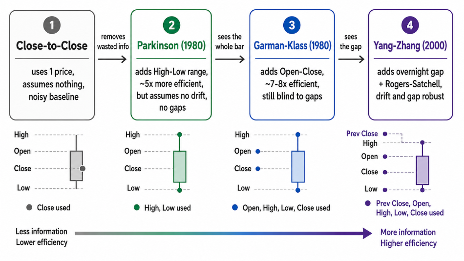
Fig. 2. From close-to-close to Yang-Zhang: the prices each estimator uses and the assumption it drops.
Building the library: CVolatilityEstimators
Why a class with a rolling buffer, and not free functions. These estimators are not recursive: each is a function of the last N complete bars, not of a single running state updated one sample at a time. We could write them as free functions over the OHLC arrays, but every one needs the same rolling window, and two of them, close-to-close and the Yang-Zhang overnight term, also need the close of the bar immediately preceding the window. Wrapping the window in a class that owns its buffer means the estimators share that storage, the caller never does index arithmetic, and the object has a clean lifecycle. The class keeps the last window + 1 bars, the extra one being the lagged close.
That storage is a ring buffer, not a shifting array: a new bar overwrites the oldest slot and a head index advances, so pushing a bar is O(1) regardless of window size. A private Slot helper maps the logical index "i bars ago" onto the physical slot, so the estimators read the window in natural order while the modular arithmetic lives in one place. Here is the file header and class declaration.
//+------------------------------------------------------------------+
//|                                        VolatilityEstimators.mqh  |
//|   Range-based OHLC volatility estimators in one reusable library |
//|                                                                  |
//|   One source of truth for the classic historical-volatility      |
//|   estimators used by the visual indicators. Feed one bar per call|
//|   with Update(open,high,low,close); read any estimate back as a  |
//|   per-bar standard deviation (Value) or an annualized figure.    |
//|                                                                  |
//|   Unlike a recursive filter, every estimator here is *windowed*: |
//|   the result is a function of the last N complete bars. The class|
//|   keeps its bars in a fixed-size RING BUFFER, so pushing a new   |
//|   bar is O(1) (no array shift) and callers never manage index    |
//|   math.                                                          |
//|                                                                  |
//|   Formulas are the standard published definitions:               |
//|     Close-to-Close  classic log-return sample variance           |
//|     Parkinson       (1980)  high-low range                       |
//|     Garman-Klass    (1980)  full OHLC bar, no overnight gap      |
//|     Yang-Zhang      (2000)  drift- and gap-independent           |
//|   Each returns sigma per bar; annualize by sqrt(bars per year).  |
//+------------------------------------------------------------------+
#property copyright "Adeolu Kayode"
#property strict

#define VOL_LN2 0.69314718055994530942   // ln(2), used by Parkinson & Garman-Klass
The ENUM_VOL_METHOD selector lets a caller switch estimator from a single input, which both indicators use. A companion SVolEstimates struct bundles all four per-bar sigmas, so an indicator that wants every estimator at once can retrieve them from a single window pass rather than four separate calls. The class itself then holds four parallel arrays for the OHLC history plus the bookkeeping integers.
//+------------------------------------------------------------------+
//| Method selector shared by the class and its callers. Passing an  |
//| enum (rather than four separate accessors) lets an indicator     |
//| switch estimator from a single input without branching by hand.  |
//+------------------------------------------------------------------+
enum ENUM_VOL_METHOD
  {
   VOL_CLOSE_TO_CLOSE = 0,  // Close-to-Close (naive log-return sigma)
   VOL_PARKINSON      = 1,  // Parkinson (high-low range)
   VOL_GARMAN_KLASS   = 2,  // Garman-Klass (full OHLC bar)
   VOL_YANG_ZHANG     = 3   // Yang-Zhang (gap- and drift-robust)
  };
//+------------------------------------------------------------------+
//| Bundle of all four per-bar sigmas from a single window pass.     |
//| ComputeAll() fills one of these so an indicator that needs every |
//| estimator (like the comparison panel) sweeps the window once     |
//| instead of four times.                                           |
//+------------------------------------------------------------------+
struct SVolEstimates
  {
   double            ctc;   // Close-to-Close sigma
   double            park;  // Parkinson sigma
   double            gk;    // Garman-Klass sigma
   double            yz;    // Yang-Zhang sigma
  };
The private section holds the ring storage, the head index, and two helpers. Slot subtracts from the head and wraps once if the result goes negative. SampleVarFromSums is the Bessel-corrected sample variance computed from a running sum and sum-of-squares rather than an array, so no temporary buffer is needed.
private:
   double            m_open[];    // fixed ring storage, physical slots (see Slot())
   double            m_high[];    //   logical "i bars ago" is mapped by Slot(i)
   double            m_low[];     //   0 = most recent bar, up to window bars back
   double            m_close[];   //   the extra slot holds the lagged close
   int               m_window;    // number of bars each estimate is computed over
   int               m_cap;       // ring capacity = window + 1 (holds the lagged close)
   int               m_count;     // real bars pushed so far (for warm-up / Ready)
   int               m_head;      // physical slot that currently holds the most recent bar

//--- map logical index (i bars ago, 0 = most recent) to a physical ring slot
   int               Slot(const int i) const
     {
      int s = m_head - i;
      if(s < 0)
         s += m_cap;
      return(s);
     }

//--- sample variance of two parallel accumulators (Bessel-corrected).
//--- Pass sum and sum-of-squares of n values; avoids a temp array.
   double            SampleVarFromSums(const double sum, const double sumsq, const int n) const
     {
      if(n < 2)
         return(0.0);
      double mean = sum / n;
      double ss   = sumsq - (double)n * mean * mean;
      if(ss < 0.0)
         ss = 0.0;
      return(ss / (n - 1));
     }
The public lifecycle mirrors the way an indicator drives it: Init sizes the ring and resets the head, Reset clears the accumulated bars without reallocating (used when an indicator replays a window), Update feeds one bar, and Ready reports when a full window has accumulated. Two details matter. First, Init allocates window + 1 slots, the extra one holding the lagged close. Second, Update validates its input, rejecting any bar with a non-positive price or a high below its low, and returns a bool so a caller can tell a bad bar was skipped. Malformed bars are skipped rather than left to corrupt every logarithm downstream. There is also a ReadyIntrabar alongside Ready: Parkinson and Garman-Klass never look at the previous close, so they are valid one bar earlier than the two estimators that do.
public:
                     CVolatilityEstimators() : m_window(20), m_cap(21), m_count(0), m_head(-1) {}

//--- set the estimation window (bars) and allocate the ring buffer
   void              Init(const int window)
     {
      m_window = (window < 2 ? 2 : window);
      m_cap    = m_window + 1;               // +1 bar supplies the previous close
      ArrayResize(m_open,  m_cap);
      ArrayResize(m_high,  m_cap);
      ArrayResize(m_low,   m_cap);
      ArrayResize(m_close, m_cap);
      ArrayInitialize(m_open,  0.0);
      ArrayInitialize(m_high,  0.0);
      ArrayInitialize(m_low,   0.0);
      ArrayInitialize(m_close, 0.0);
      m_count = 0;
      m_head  = -1;                           // no bar yet; first Update() lands in slot 0
     }

//--- discard accumulated bars but keep the window/allocation. Cheap
//--- reset used when replaying a fresh window without reallocating.
   void              Reset()
     {
      m_count = 0;
      m_head  = -1;
     }

//--- feed one completed bar; call once per bar in chart order.
//--- Malformed bars (non-positive price, or high<low) are rejected
//--- so a single bad tick cannot poison the logarithms downstream.
//--- Returns true if the bar was accepted.
   bool              Update(const double o, const double h, const double l, const double c)
     {
      if(o <= 0.0 || h <= 0.0 || l <= 0.0 || c <= 0.0 || h < l)
         return(false);
      m_head = (m_head + 1) % m_cap;          // advance ring head, overwriting oldest slot
      m_open[m_head]  = o;
      m_high[m_head]  = h;
      m_low[m_head]   = l;
      m_close[m_head] = c;
      if(m_count < m_cap)
         m_count++;
      return(true);
     }

//--- true once a full window (plus the lagged close) has been seen.
//--- window+1 bars are the requirement for the two estimators that
//--- reference the previous close (Close-to-Close, Yang-Zhang overnight).
   bool              Ready() const { return(m_count >= m_cap); }

//--- Parkinson and Garman-Klass need only 'window' bars (no lagged
//--- close). Expose it so a caller can start those two one bar early.
   bool              ReadyIntrabar() const { return(m_count >= m_window); }
The estimators themselves. Each guards on its readiness check, then implements its formula directly over the ring buffer through Slot. Close-to-close is the simplest: it accumulates the sum and sum-of-squares of the log returns and hands them to SampleVarFromSums. Note Slot(i + 1), which reaches the bar before the window, exactly why the ring holds one extra slot.
//--- Close-to-Close: sample standard deviation of log returns
//--- r = ln(C_t / C_{t-1}) over the window. Accumulates sum and
//--- sum-of-squares in one pass, so no temporary array is allocated.
   double            CloseToClose() const
     {
      if(!Ready())
         return(0.0);
      double sum = 0.0, sumsq = 0.0;
      for(int i = 0; i < m_window; i++)          // i bars back within the window
        {
         double r = MathLog(m_close[Slot(i)] / m_close[Slot(i + 1)]);
         sum   += r;
         sumsq += r * r;
        }
      return(MathSqrt(SampleVarFromSums(sum, sumsq, m_window)));
     }
Parkinson and Garman-Klass are single accumulation loops that translate their formulas line for line, with VOL_LN2 supplying the 4 ln2 normalizer and the (2 ln2 - 1) weight. Both gate on ReadyIntrabar, since neither touches the previous close, and Garman-Klass takes the square root only when its variance is positive, guarding the rare negative from noisy data.
//--- Parkinson (1980): uses the high-low range of each bar.
   double            Parkinson() const
     {
      if(!ReadyIntrabar())
         return(0.0);
      double sum = 0.0;
      for(int i = 0; i < m_window; i++)
        {
         int s = Slot(i);
         double hl = MathLog(m_high[s] / m_low[s]);
         sum += hl * hl;
        }
      return(MathSqrt(sum / (4.0 * m_window * VOL_LN2)));
     }

//--- Garman-Klass (1980): combines the high-low range with the
//--- open-close move, using the whole bar.
   double            GarmanKlass() const
     {
      if(!ReadyIntrabar())
         return(0.0);
      double sum = 0.0;
      for(int i = 0; i < m_window; i++)
        {
         int s = Slot(i);
         double hl = MathLog(m_high[s] / m_low[s]);
         double co = MathLog(m_close[s] / m_open[s]);
         sum += 0.5 * hl * hl - (2.0 * VOL_LN2 - 1.0) * co * co;
        }
      double var = sum / m_window;
      return(var > 0.0 ? MathSqrt(var) : 0.0);
     }
Yang-Zhang is the one with real structure. In a single pass over the window it accumulates the overnight returns, the open-to-close returns, and the Rogers-Satchell sum, then blends the three variances with the weight k. This is the method the bands indicator calls.
//--- Yang-Zhang (2000): the only one of the four that is both drift
//--- and gap-independent. One pass accumulates the overnight and
//--- open-to-close variances (via running sums) and the Rogers-
//--- Satchell term, so no temporary arrays are allocated.
   double            YangZhang() const
     {
      if(!Ready())
         return(0.0);

      double on_sum = 0.0, on_sq = 0.0;   // overnight   ln(O_t / C_{t-1})
      double oc_sum = 0.0, oc_sq = 0.0;   // open-close  ln(C_t / O_t)
      double rs     = 0.0;                // Rogers-Satchell (mean-of-products form)

      for(int i = 0; i < m_window; i++)
        {
         int s  = Slot(i);
         int sp = Slot(i + 1);            // previous bar (the lagged close)

         double on = MathLog(m_open[s]  / m_close[sp]);
         double oc = MathLog(m_close[s] / m_open[s]);
         on_sum += on;
         on_sq  += on * on;
         oc_sum += oc;
         oc_sq  += oc * oc;

         double hc = MathLog(m_high[s] / m_close[s]);
         double ho = MathLog(m_high[s] / m_open[s]);
         double lc = MathLog(m_low[s]  / m_close[s]);
         double lo = MathLog(m_low[s]  / m_open[s]);
         rs += hc * ho + lc * lo;
        }
      double sigma_on = SampleVarFromSums(on_sum, on_sq, m_window);   // overnight variance
      double sigma_oc = SampleVarFromSums(oc_sum, oc_sq, m_window);   // open-to-close variance
      double sigma_rs = rs / m_window;                                // Rogers-Satchell variance

      double k = 0.34 / (1.34 + (double)(m_window + 1) / (m_window - 1));
      double var = sigma_on + k * sigma_oc + (1.0 - k) * sigma_rs;
      return(var > 0.0 ? MathSqrt(var) : 0.0);
     }
Calling all four estimators one after another sweeps the window four times. ComputeAll folds every accumulation into one loop and finishes each with its own normalizer, so the comparison indicator touches each bar once no matter how many estimators it draws.
//--- Compute all four estimators for the current window. Parkinson,
//--- Garman-Klass and Yang-Zhang share a single sweep of the bars;
//--- Close-to-Close (which needs only the closes) is folded into the
//--- same loop. One pass instead of four separate ones.
   bool              ComputeAll(SVolEstimates &out) const
     {
      out.ctc = 0.0;
      out.park = 0.0;
      out.gk = 0.0;
      out.yz = 0.0;
      if(!Ready())
         return(false);

      double c_sum = 0.0, c_sq = 0.0;     // close-to-close log returns
      double on_sum = 0.0, on_sq = 0.0;   // Yang-Zhang overnight
      double oc_sum = 0.0, oc_sq = 0.0;   // Yang-Zhang open-to-close
      double park = 0.0;                  // Parkinson high-low accumulator
      double gk   = 0.0;                  // Garman-Klass accumulator
      double rs   = 0.0;                  // Rogers-Satchell accumulator

      for(int i = 0; i < m_window; i++)
        {
         int s  = Slot(i);
         int sp = Slot(i + 1);

         double hl = MathLog(m_high[s] / m_low[s]);
         double co = MathLog(m_close[s] / m_open[s]);
         double r  = MathLog(m_close[s] / m_close[sp]);
         double on = MathLog(m_open[s]  / m_close[sp]);

         c_sum  += r;
         c_sq  += r * r;
         on_sum += on;
         on_sq += on * on;
         oc_sum += co;
         oc_sq += co * co;

         park += hl * hl;
         gk   += 0.5 * hl * hl - (2.0 * VOL_LN2 - 1.0) * co * co;

         double hc = MathLog(m_high[s] / m_close[s]);
         double ho = MathLog(m_high[s] / m_open[s]);
         double lc = MathLog(m_low[s]  / m_close[s]);
         double lo = MathLog(m_low[s]  / m_open[s]);
         rs += hc * ho + lc * lo;
        }

      out.ctc  = MathSqrt(SampleVarFromSums(c_sum, c_sq, m_window));
      out.park = MathSqrt(park / (4.0 * m_window * VOL_LN2));

      double gk_var = gk / m_window;
      out.gk = (gk_var > 0.0 ? MathSqrt(gk_var) : 0.0);

      double sigma_on = SampleVarFromSums(on_sum, on_sq, m_window);
      double sigma_oc = SampleVarFromSums(oc_sum, oc_sq, m_window);
      double sigma_rs = rs / m_window;
      double k = 0.34 / (1.34 + (double)(m_window + 1) / (m_window - 1));
      double yz_var = sigma_on + k * sigma_oc + (1.0 - k) * sigma_rs;
      out.yz = (yz_var > 0.0 ? MathSqrt(yz_var) : 0.0);
      return(true);
     }
Finally, two accessors: Value dispatches on the enum to select an estimator at runtime, and Annualized scales a per-bar sigma by the square root of the bars per year.
//--- per-bar sigma for the requested estimator
   double            Value(const ENUM_VOL_METHOD method) const
     {
      switch(method)
        {
         case VOL_CLOSE_TO_CLOSE:
            return(CloseToClose());
         case VOL_PARKINSON:
            return(Parkinson());
         case VOL_GARMAN_KLASS:
            return(GarmanKlass());
         case VOL_YANG_ZHANG:
            return(YangZhang());
        }
      return(0.0);
     }

//--- scale a per-bar sigma to an annualized figure (barsPerYear e.g. 252)
   double            Annualized(const ENUM_VOL_METHOD method, const double barsPerYear) const
     {
      return(Value(method) * MathSqrt(barsPerYear));
     }
That is the entire library: no state beyond the ring buffer and its head index, and no external dependency. Each estimator implements its published formula, wrapped in a few deliberate decisions, Bessel-corrected variances, a readiness rule aligned to the most demanding estimator, running-sum accumulation, and annualization kept outside the estimator. The two indicators that follow are thin drivers over this class.
Indicator 1: seeing the efficiency difference
The efficiency argument is easy to state and much more convincing to see. The first indicator plots all four estimators in a separate window, on the same annualized axis, so the difference in smoothness is immediate. It is a thin driver: feed the class each bar of the recomputed tail, pull all four estimates back with a single ComputeAll, and write them into four buffers.
The visual design does part of the teaching. The #property block requests a separate window and four line plots, with deliberate colors: close-to-close in muted silver so its noise reads as a grey haze, the two intrabar estimators in equal-weight colors, and Yang-Zhang in double width as the line to follow. The finished chart shows one busy grey line and three calmer colored ones.
#property indicator_separate_window
#property indicator_buffers 4
#property indicator_plots   4

#property indicator_label1  "Close-to-Close"
#property indicator_type1   DRAW_LINE
#property indicator_color1  clrSilver
#property indicator_width1  1

#property indicator_label2  "Parkinson"
#property indicator_type2   DRAW_LINE
#property indicator_color2  clrMediumSeaGreen
#property indicator_width2  1

#property indicator_label3  "Garman-Klass"
#property indicator_type3   DRAW_LINE
#property indicator_color3  clrGoldenrod
#property indicator_width3  1

#property indicator_label4  "Yang-Zhang"
#property indicator_type4   DRAW_LINE
#property indicator_color4  clrDodgerBlue
#property indicator_width4  2
The inputs are the estimation window and the annualization factor, and the four indicator buffers, one per estimator, are declared as globals alongside a single instance of our library class.
#include <Volatility/VolatilityEstimators.mqh>

input int    InpWindow      = 20;     // Estimation window (bars)
input double InpBarsPerYear = 252.0;  // Bars per year for annualization (0 = raw per-bar sigma)

double CtcBuffer[];   // Close-to-Close sigma
double ParkBuffer[];  // Parkinson sigma
double GkBuffer[];    // Garman-Klass sigma
double YzBuffer[];    // Yang-Zhang sigma

CVolatilityEstimators g_vol;   // rolling-window estimator engine
OnInit binds each buffer to its plot index, sizes the estimator to the requested window, and sets a short name. The short name is the display name MetaTrader shows for the indicator, and building it with IndicatorSetString so it echoes the window means you can tell at a glance which parameters an instance is running with. We also set five digits of display precision, appropriate for the small annualized-sigma values.
//+------------------------------------------------------------------+
//| Custom indicator initialization function                         |
//+------------------------------------------------------------------+
int OnInit()
  {
   SetIndexBuffer(0, CtcBuffer,  INDICATOR_DATA);
   SetIndexBuffer(1, ParkBuffer, INDICATOR_DATA);
   SetIndexBuffer(2, GkBuffer,   INDICATOR_DATA);
   SetIndexBuffer(3, YzBuffer,   INDICATOR_DATA);

   g_vol.Init(InpWindow);
   IndicatorSetString(INDICATOR_SHORTNAME, StringFormat("VolCompare(%d)", InpWindow));
   IndicatorSetInteger(INDICATOR_DIGITS, 5);
   return(INIT_SUCCEEDED);
  }
The calculation is driven by prev_calculated, so it does the minimum work each call. The first pass computes every bar; every later tick recomputes only the tail, starting one bar back so the last (possibly unclosed) bar is refreshed. The ring is re-seeded with the window + 1 bars before that point, so the first written bar already has a full window, and a single ComputeAll per bar fills all four estimators from one pass. Bars before the window fills are set to EMPTY_VALUE during warm-up.
//+------------------------------------------------------------------+
//| Incremental calculation driven by prev_calculated.               |
//|                                                                  |
//| On the first pass (or a history refresh) prev_calculated is 0    |
//| and we recompute the whole series. On every later tick only the  |
//| tail has changed, so we recompute from 'start': the previously   |
//| last bar (which may have been unclosed) plus everything after it.|
//| The ring buffer is re-seeded with the window+1 bars that precede |
//| 'start' so the first written bar already has a full window, then |
//| a single ComputeAll() per bar fills all four estimators at once. |
//+------------------------------------------------------------------+
int OnCalculate(const int rates_total,
                const int prev_calculated,
                const datetime &time[],
                const double &open[],
                const double &high[],
                const double &low[],
                const double &close[],
                const long &tick_volume[],
                const long &volume[],
                const int &spread[])
  {
   if(rates_total < InpWindow + 2)
      return(0);

//--- annualization scale (1.0 keeps the raw per-bar sigma when disabled)
   double scale = (InpBarsPerYear > 0.0 ? MathSqrt(InpBarsPerYear) : 1.0);

//--- first bar we must (re)write: the previously last bar, or 0 on a fresh pass
   int start = (prev_calculated > 0 ? prev_calculated - 1 : 0);

//--- re-seed the ring with the (window+1) bars preceding 'start' so the
//--- window is already full when we begin writing. 'seed' is clamped to 0.
   int seed = start - (InpWindow + 1);
   if(seed < 0)
      seed = 0;

   g_vol.Reset();
   for(int i = seed; i < start; i++)
      g_vol.Update(open[i], high[i], low[i], close[i]);

   SVolEstimates e;
   for(int i = start; i < rates_total; i++)
     {
      g_vol.Update(open[i], high[i], low[i], close[i]);
      if(g_vol.ComputeAll(e))
        {
         CtcBuffer[i]  = e.ctc  * scale;
         ParkBuffer[i] = e.park * scale;
         GkBuffer[i]   = e.gk   * scale;
         YzBuffer[i]   = e.yz   * scale;
        }
      else
        {
         CtcBuffer[i]  = EMPTY_VALUE;
         ParkBuffer[i] = EMPTY_VALUE;
         GkBuffer[i]   = EMPTY_VALUE;
         YzBuffer[i]   = EMPTY_VALUE;
        }
     }
   return(rates_total);
  }
On a chart, the result makes the whole argument for you.
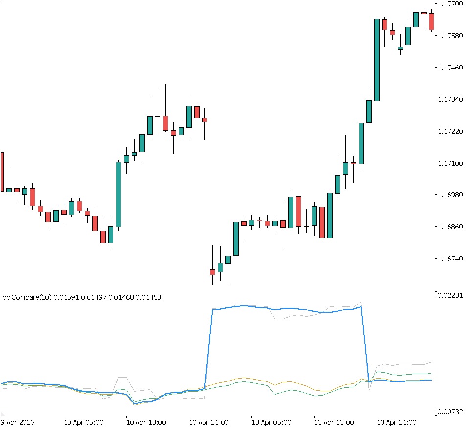
Fig. 3. VolatilityComparison on [SYMBOL, TIMEFRAME]. Close-to-Close (silver) is the noisiest; the range estimators track more smoothly; Yang-Zhang (blue) lifts on gaps.
Indicator 2: gap-aware volatility bands
The comparison indicator is a teaching tool. The second indicator is something you might actually trade with: volatility bands, like Bollinger Bands, but with the band width driven by the Yang-Zhang estimator instead of the standard deviation of closes. Because Yang-Zhang measures the overnight gap directly, the channel widens correctly right after a weekend or session jump, where a plain standard-deviation band stays narrow until the gap has already worked its way into the closing-price window.
Unlike the comparison indicator, this one draws on the price chart itself, so the #property block requests the chart window rather than a separate one, and declares three plots: the upper and lower bands in the same color so they read as a channel, and a dotted middle line for the center.
#property indicator_chart_window
#property indicator_buffers 3
#property indicator_plots   3

#property indicator_label1  "Upper"
#property indicator_type1   DRAW_LINE
#property indicator_color1  clrCrimson
#property indicator_width1  1

#property indicator_label2  "Middle"
#property indicator_type2   DRAW_LINE
#property indicator_color2  clrDimGray
#property indicator_width2  1
#property indicator_style2  STYLE_DOT

#property indicator_label3  "Lower"
#property indicator_type3   DRAW_LINE
#property indicator_color3  clrCrimson
#property indicator_width3  1
The inputs separate the volatility window from the MA period, so you can smooth the center independently of the volatility measurement, and expose the band multiplier. Alongside the three buffers we keep a g_warmup integer, whose purpose becomes clear in the initialization below.
#include <Volatility/VolatilityEstimators.mqh>

input int    InpWindow     = 20;    // Volatility window (bars)
input int    InpMAPeriod   = 20;    // Center moving-average period (bars)
input double InpMultiplier = 2.0;   // Band width in standard deviations

double UpperBuffer[];   // center * exp(+mult*sigma)
double MiddleBuffer[];  // simple moving average of close (channel center)
double LowerBuffer[];   // center * exp(-mult*sigma)

CVolatilityEstimators g_vol;   // rolling-window estimator engine
int g_warmup;                  // first bar index with both MA and volatility ready
OnInit binds the three buffers and computes the warm-up boundary. The indicator cannot draw until both ingredients are ready: the volatility estimate (which needs InpWindow + 1 bars) and the moving average (ready at index InpMAPeriod - 1, hence the asymmetric terms, since these are bar indices, not counts). The MathMax of the two means whichever fills last governs the first drawable bar, so we never plot a band with a half-formed center or width.
//+------------------------------------------------------------------+
//| Custom indicator initialization function                         |
//+------------------------------------------------------------------+
int OnInit()
  {
   SetIndexBuffer(0, UpperBuffer,  INDICATOR_DATA);
   SetIndexBuffer(1, MiddleBuffer, INDICATOR_DATA);
   SetIndexBuffer(2, LowerBuffer,  INDICATOR_DATA);

   g_vol.Init(InpWindow);
   g_warmup = MathMax(InpWindow + 1, InpMAPeriod - 1);   // both inputs must be filled
   IndicatorSetString(INDICATOR_SHORTNAME,
                      StringFormat("VolBands(%d,%d,%.1f)", InpWindow, InpMAPeriod, InpMultiplier));
   IndicatorSetInteger(INDICATOR_DIGITS, _Digits);
   return(INIT_SUCCEEDED);
  }
The center line is a simple moving average of the close. Rather than re-summing the whole period on every bar, the calculation below keeps a rolling sum: it is seeded once for the first bar of the recomputed tail, then advanced by adding the new close and subtracting the one that just fell out of the window. The helper below does only the one-off seeding, returning the sum of the period closes ending at bar i.
//+------------------------------------------------------------------+
//| Simple moving average of the InpMAPeriod closes ending at i,     |
//| computed directly. Used once per recalculated tail to seed the   |
//| rolling sum; the loop below then maintains it in O(1) per bar.   |
//+------------------------------------------------------------------+
double SmaSum(const double &close[], const int i, const int period)
  {
   double sum = 0.0;
   for(int k = 0; k < period; k++)
      sum += close[i - k];
   return(sum);
  }
The full calculation is below. Its structure mirrors the comparison indicator: it is driven by prev_calculated, recomputes only the tail from start, and re-seeds the Yang-Zhang ring with the window + 1 bars before it. Here start is also clamped to the warm-up boundary, so nothing is drawn before both the volatility window and the moving average are full. Alongside the ring, the moving-average sum is seeded once with SmaSum and then rolled forward one bar at a time. The band construction at the bottom deserves close attention.
//+------------------------------------------------------------------+
//| Incremental calculation driven by prev_calculated.               |
//|                                                                  |
//| Only the tail is recomputed on each tick: from 'start' (the      |
//| previously last bar, possibly unclosed) to the end. The Yang-    |
//| Zhang ring buffer is re-seeded with the window+1 preceding bars, |
//| and the center's moving-average sum is kept as a rolling sum so  |
//| each bar costs O(1) instead of re-summing InpMAPeriod closes.    |
//+------------------------------------------------------------------+
int OnCalculate(const int rates_total,
                const int prev_calculated,
                const datetime &time[],
                const double &open[],
                const double &high[],
                const double &low[],
                const double &close[],
                const long &tick_volume[],
                const long &volume[],
                const int &spread[])
  {
   if(rates_total < g_warmup + 1)
      return(0);

//--- first bar we must (re)write; never before the warm-up boundary
   int start = (prev_calculated > 0 ? prev_calculated - 1 : 0);
   if(start < g_warmup)
      start = g_warmup;

//--- re-seed the Yang-Zhang ring with the (window+1) bars before 'start'
   int seed = start - (InpWindow + 1);
   if(seed < 0)
      seed = 0;
   g_vol.Reset();
   for(int i = seed; i < start; i++)
      g_vol.Update(open[i], high[i], low[i], close[i]);

//--- rolling moving-average sum of the InpMAPeriod closes ending at 'start'
   double ma_sum = SmaSum(close, start, InpMAPeriod);

   for(int i = start; i < rates_total; i++)
     {
      if(i > start)
         ma_sum += close[i] - close[i - InpMAPeriod];

      g_vol.Update(open[i], high[i], low[i], close[i]);

      if(!g_vol.Ready())
        {
         UpperBuffer[i]  = EMPTY_VALUE;
         MiddleBuffer[i] = EMPTY_VALUE;
         LowerBuffer[i]  = EMPTY_VALUE;
         continue;
        }

      //--- center line and the per-bar Yang-Zhang sigma (a log-return sd)
      double center = ma_sum / InpMAPeriod;
      double sigma  = g_vol.YangZhang();
      double offset = InpMultiplier * sigma;

      //--- exact multiplicative bands: sigma is a log-return sd, so the
      //--- price offset is center*(exp(+/-offset)-1). This keeps the upper
      //--- and lower bands correctly asymmetric in price at larger sigma.
      MiddleBuffer[i] = center;
      UpperBuffer[i]  = center * MathExp(offset);
      LowerBuffer[i]  = center * MathExp(-offset);
     }
   return(rates_total);
  }
The band construction deserves attention. The Yang-Zhang output is a standard deviation of log returns, a dimensionless quantity, not a price, so the right way to turn it into bands is a proportional move: the center times the exponential of the positive offset for the upper band, of the negative offset for the lower. That makes the bands correctly asymmetric at larger sigma, the upper sitting slightly further from the center than the lower, exactly as a lognormal price distribution implies. Simply adding and subtracting a price amount is the naive shortcut, and it is wrong for anything but very small sigma.
On the chart, the bands behave like Bollinger Bands in calm conditions but diverge from them exactly where it matters.
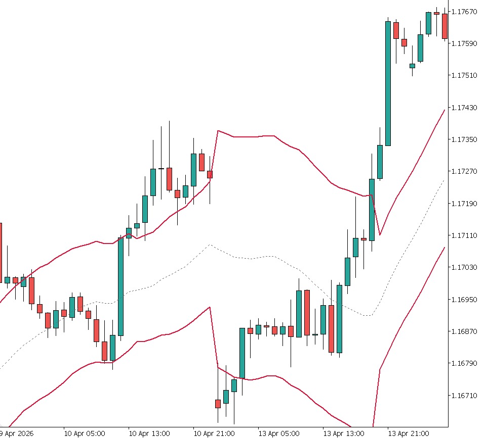
Fig. 4. VolatilityBands on [SYMBOL, TIMEFRAME]. The channel widens on the gap bar itself.
The claim that these bands react to a gap sooner than a standard-deviation band is worth demonstrating directly. Placing our Yang-Zhang bands and the platform's built-in Bollinger Bands on the same chart, with the same period and multiplier, makes the difference concrete: on the bar that gaps, the Yang-Zhang channel is already wide, while the Bollinger channel only catches up over the following bars as the jump filters into its closing-price window.
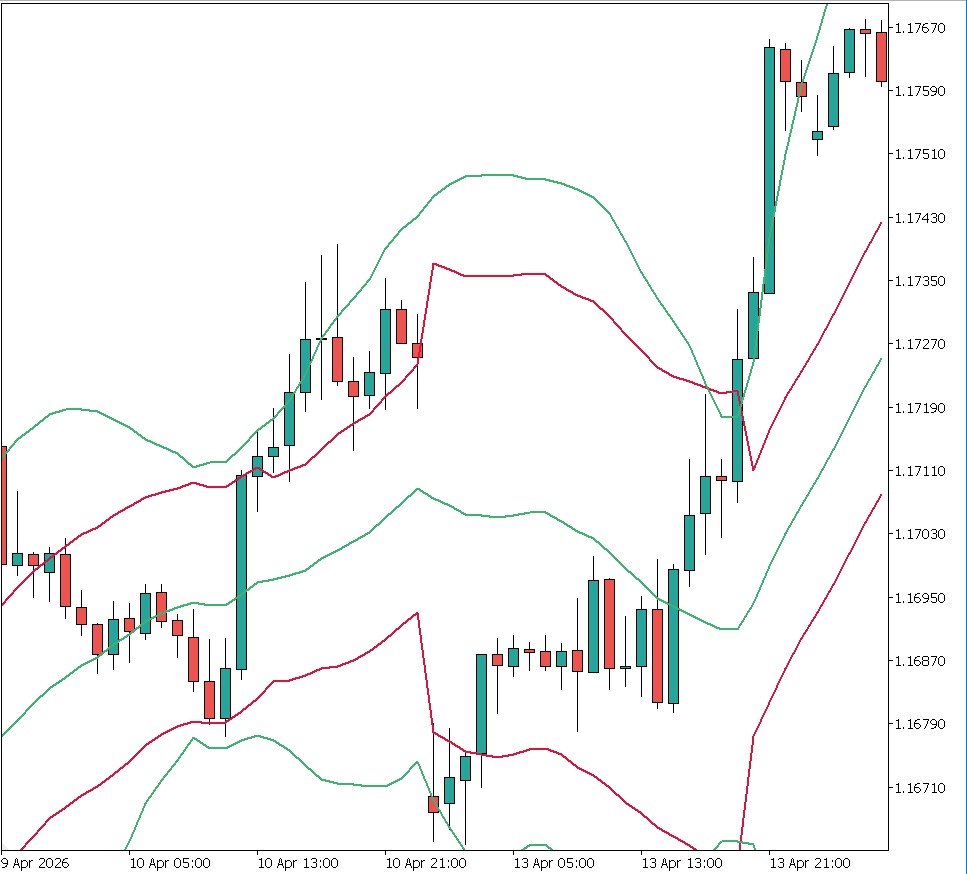
Fig. 5. Yang-Zhang bands (red) vs. Bollinger Bands (blue), same settings. Yang-Zhang widens on the gap bar; Bollinger reacts several bars later.
Edge cases and pitfalls
The formulas are simple, but using these estimators correctly on live markets involves a few decisions that the math alone does not settle. This section is the part no reference contains, and it is where most of the practical value lives.
The annualization factor is not universal. Both indicators default to 252, the number of trading days in a year, which is correct only if each bar is one trading day. Annualization scales a per-bar sigma by the square root of the number of bars per year, so on an H1 chart of a market trading 24 hours, five days a week, the right factor is closer to 6240 (24 times 5 times 52), not 252. If you leave it at 252 on an intraday chart, the absolute numbers are meaningless, though the relative comparison between estimators still holds because they are all scaled by the same constant. Set this deliberately to the bars-per-year of your actual timeframe, or set it to 0 and read the raw per-bar sigma.
The overnight-gap term depends on your instrument's session structure. Yang-Zhang's advantage is that it measures the open-to-previous-close gap. But what counts as a "gap" depends entirely on how the broker builds bars. On spot forex, which trades continuously from Sunday evening to Friday, consecutive intraday bars have essentially no gap, so the overnight term is near zero except across the weekend, and Yang-Zhang converges toward the pure intrabar estimators. On stocks, indices, and futures with real session breaks, the overnight term carries genuine information and Yang-Zhang's advantage is largest. In other words, the more your instrument gaps, the more reason to prefer Yang-Zhang, and on a near-continuous instrument the cheaper Garman-Klass is barely distinguishable.
Watch for zero or malformed bars. Every estimator takes logarithms of price ratios, so a bar with a zero or negative price, or a high below its low from bad tick data, would produce a NaN that propagates. The class guards against this directly: Update rejects any bar with a non-positive price or an inverted high and low, and returns false so a caller can detect the skip. Real broker data is almost always clean, but if you feed these estimators synthetic or imported data, a rejected bar simply does not enter the window, which is safer than letting one poisoned value corrupt the whole estimate.
Warm-up and the window plus one. Both indicators produce nothing until Ready returns true, which needs window + 1 bars because of the lagged close. On a fresh chart with little history, or a very large window, expect a blank region on the left. This is correct behavior, not a bug.
The incremental recalculation is exact. The tail-only recomputation re-seeds the ring with the preceding window + 1 bars. Therefore, the result on every bar matches a full replay, but at lower cost. If you extend the class, preserve that invariant: the seed window must be at least window + 1 bars, or the first recomputed bar starts from an incomplete window.
Drift over short windows. Rogers-Satchell, and therefore Yang-Zhang, is specifically built to stay unbiased when the price drifts. Parkinson and Garman-Klass are not: on a strongly trending window they will read slightly low, because a steady drift inflates the range without adding the kind of variance they assume. Over the short windows typical of an indicator this bias is usually small, but it is another reason Yang-Zhang is the safer default when you are unsure.
Using the library in your own code
The two indicators are the visual demonstration, but the point of a library is that you can call it from anywhere. Using it from an Expert Advisor is the same three-step lifecycle the indicators follow, only without the drawing: create the object, feed it one completed bar per new bar, and read a value back once it is ready. A minimal skeleton looks like this.
#include <Volatility/VolatilityEstimators.mqh>

CVolatilityEstimators vol;

int OnInit()
  {
   vol.Init(20);                     // 20-bar estimation window
   return(INIT_SUCCEEDED);
  }

//--- call once per completed bar (e.g. from an OnTick new-bar guard)
void OnNewBar()
  {
//--- feed the last CLOSED bar (shift 1), never the forming bar (shift 0)
   vol.Update(iOpen(_Symbol, _Period, 1),
             iHigh(_Symbol, _Period, 1),
             iLow(_Symbol, _Period, 1),
             iClose(_Symbol, _Period, 1));

   if(vol.Ready())
     {
      double yz = vol.YangZhang();       // per-bar sigma
      // use yz as a volatility-regime filter, or scale position size by 1/yz
     }
  }
Two things matter in that skeleton. First, feed the class the last closed bar (shift 1), not the forming bar (shift 0), so that each estimate is built from finalized OHLC and does not jitter within the bar. Second, call Update exactly once per bar, which is what a new-bar guard in OnTick gives you; if you want a value from a specific estimator rather than Yang-Zhang, call Value(VOL_GARMAN_KLASS) and so on, or Annualized(method, barsPerYear) for a comparable annual figure. That single returned number is exactly what a regime filter or an inverse-volatility position sizer needs.
Which estimator should you actually pick? The earlier table lists what each one uses and assumes. This one is blunter: it maps a situation straight to a choice.
| Market or use case | Recommended estimator |
|---|---|
| Daily stocks, indices, or futures with session gaps | Yang-Zhang |
| Intraday forex or any near-continuous market | Garman-Klass, or Yang-Zhang (they nearly coincide) |
| A baseline comparable to classic historical volatility | Close-to-Close |
| The simplest range-only measure | Parkinson |
One caveat on that table, because Yang-Zhang is not magically always the best. On truly continuous intraday data, where each bar's open sits right on the previous close, its overnight term contributes almost nothing and it converges to Garman-Klass, so the extra machinery buys little. And over very short windows every estimator here is noisy, range-based or not, because there simply are not enough bars to average out. Yang-Zhang is the safest default, not a universal winner; the point of shipping all four behind one enum is that switching costs you a single input.
Performance, in one breath. Three design choices keep the cost down. The ring buffer makes each bar's insertion O(1), with no array shift. ComputeAll produces all four estimates from a single sweep of the window instead of four separate passes. And prev_calculated makes recalculation tail-only, so per-tick work does not grow with history length. Together they take the class from a demonstration to something you can leave running on many charts, or inside a tester, without a second thought.
Conclusion
We set out to close a real gap in the MetaTrader 5 tool set: the classic range-based volatility estimators, famous in the literature and absent from the platform. We built VolatilityEstimators.mqh, a single dependency-free library implementing Close-to-Close, Parkinson, Garman-Klass, and Yang-Zhang behind one rolling-window class that is built to be reused, not just demonstrated: an O(1) ring buffer, allocation-free estimators, a one-pass ComputeAll, and input validation at the boundary. We then used it to build two indicators, both driven incrementally through prev_calculated, a comparison panel that makes the efficiency difference visible, and a set of gap-aware volatility bands that put the best of the four to practical use.
More than the code, the takeaway is the reasoning: each estimator is defined by the assumption it makes about the market, and choosing the right one is a matter of matching that assumption to your instrument. Close-to-close wastes information but assumes nothing. Parkinson and Garman-Klass are highly efficient but blind to gaps and drift. Yang-Zhang costs a little peak efficiency to buy robustness to both, which makes it the safest default on real, gapping, trending markets, while on a near-continuous instrument it converges to Garman-Klass and the choice barely matters. You now have all four in a form you can drop into any indicator, Expert Advisor, or research script, and the understanding to know which one to call.
A natural next step, and a good candidate for a follow-up, is to drive decisions with these estimates rather than only display them: a volatility-regime filter that blocks trades when Yang-Zhang volatility is in its top percentile, or position sizing scaled by the inverse of the estimate. The library is already shaped for that use, one call returns the number you need.
Files attached to the article
| File | Path | Description |
|---|---|---|
| VolatilityEstimators.mqh | MQL5/Include/Volatility/ | The library: four range-based volatility estimators behind one rolling-window class. |
| VolatilityComparison.mq5 | MQL5/Indicators/Volatility/ | Separate-window indicator plotting all four estimators together for comparison. |
| VolatilityBands.mq5 | MQL5/Indicators/Volatility/ | Main-chart indicator drawing gap-aware volatility bands sized by Yang-Zhang. |
| MQL5.zip | Terminal installation directory | Archive with all files above. Unpack it into the terminal installation directory and every file is placed in its required location. |
Warning: All rights to these materials are reserved by MetaQuotes Ltd. Copying or reprinting of these materials in whole or in part is prohibited.
This article was written by a user of the site and reflects their personal views. MetaQuotes Ltd is not responsible for the accuracy of the information presented, nor for any consequences resulting from the use of the solutions, strategies or recommendations described.

 Neural Networks in Trading: Effective Feature Extraction for Accurate Classification (Mantis)
 Neural Networks in Trading: Generalizing Time Series Without Data-Specific Dependence (Core Model Modules)
 Real-Time Trade Event Logger to SQLite via MQL5 DLL Bridge
 Developing a Terminal Manager (Part 2): Running Multiple Terminal Instances

- Free trading apps
- Over 8,000 signals for copying
- Economic news for exploring financial markets
You agree to website policy and terms of use