Neural Networks in Trading: Generalizing Time Series Without Data-Specific Dependence (Mamba4Cast)

Introduction

The market is both relentless and unpredictable. It offers no second chances to those who misread its signals. This is especially true today, when news spreads faster than a candlestick can form on a one-minute chart. Modern traders no longer work with the past — they work with what is only beginning to emerge from the data stream. Identifying an emerging pattern before everyone else means gaining a competitive edge. Consequently, the requirement for today's algorithms is to predict events before they become obvious, while ideally avoiding the technical burden of extensive model tuning and maintenance.

In this race, traditional models, particularly recurrent architectures, are beginning to show their limitations. They are great at recognizing repetitive patterns and retaining sequential information, yet they often struggle with the chaotic behavior of real markets. They have difficulty capturing impulses, handle poorly with gaps and outliers, and require adaptation for every new environment. Today's markets demand a more flexible and predictive solution.

Transformer-based architectures have significantly improved forecasting accuracy, particularly for long-horizon time series. However, these have come at the cost of increased computational complexity and architectural overhead. As datasets grow larger and forecasting horizons become longer, these models become progressively less suitable for real-time applications. In practice, this means more resources, longer times, and greater operational complexity.

Against this backdrop, the Mamba4Cast framework was introduced in the paper "Mamba4Cast: Efficient Zero-Shot Time Series Forecasting with State Space Models". Its design is built upon two key ideas: the lightweight yet expressive Mamba architecture and the revolutionary concept of Prior-data Fitted Networks (PFNs). Together, they establish the foundation for new approaches to time series forecasting, particularly in highly dynamic domains such as trading.

The PFN concept represents a fundamental change in thinking. Unlike conventional approaches, where a model is first pretrained on one dataset and then extensively fine-tuned on another, PFNs propose pretraining the model on a vast collection of synthetically generated tasks. Instead of learning from one real-world problem, the model learns from millions of diverse — albeit imperfect — scenarios. This makes it truly versatile and robust to new data. In trading, this means the model is not tied to a specific financial instrument or timeframe; instead, it can adapt on the fly.

The Mamba4Cast framework fully embraces the PFN philosophy. Using synthetically generated data covering a wide variety of market scenarios, it develops a broad behavioral scope. As a result, the model gets something akin to intuition — the ability to generalize patterns even under conditions of high volatility and unstable dynamics.

The second defining feature is the Mamba architecture, which exhibits linear computational complexity with respect to sequence length. Unlike Transformers, Mamba does not require quadratic operations with attention matrices and can therefore process long input sequences efficiently and economically. Most importantly for traders, Mamba4Cast predicts an entire forecasting window in a single pass. This dramatically reduces errors occurring during autoregressive forecasting while enabling faster responses to changing market conditions.

Furthermore, because the model creates multi-step forecasts, it is ideally suited for building end-to-end trading systems — from signal analysis to direct trading decision making. Mamba4Cast can become not just a guideline, but a full-fledged core of a predictive model in an automated trading system.

The Mamba4Cast Framework Algorithm

The Mamba4Cast framework represents a bold and promising step forward in the evolution of time-series forecasting systems. At its core lies a combination of rigorous mathematical foundations and flexible deep learning algorithms capable of treating markets as complex ecosystems in which past, present, and future are interconnected.

Traditional models are typically trained on the historical data of a single asset and then reproduce the relationships they have learned. This approach produced excellent results in the past, but today it faces limitations: markets are becoming more dynamic and events are becoming less predictable. Mamba4Cast takes a different approach: instead of memorizing specific historical time series, it uses the Prior-data Fitted Networks (PFN) methodology. Imagine training an analyst not on real quotes of a single stock, but on countless synthetic scenarios: trends, sideways markets, calm periods preceding major volatility spikes, and sudden news-driven shocks. This builds a universal market intelligence capable of operating out of the box on any instrument.

At the heart of the system lies the Mamba architecture, based on State Space Modeling. Unlike the intensive Self-Attention layers in Transformers, Mamba works linearly along the sequence length, enabling it to process hundreds or even thousands of time steps without an exponential increase in computational cost. This efficiency not only speeds up computation but also enables real-time market analysis, where every millisecond matters. The resulting architecture is computationally economical and well suited for processing high-frequency streaming data under volatile market conditions.

The first stage performs scaling of the input time series, using standard Min-Max normalization, where each value xt is transformed according to the following equation:

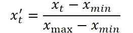
where xmin and xmax are computed over the range in the training dataset. This removes scale discrepancies between features and prepares the data for efficient learning.

Then comes the key part of preprocessing: positional encoding. Timestamps, including minute, hour, day of the week, day of the month, month, and year, are extracted separately and converted into vector representations. The algorithm uses a sinusoidal encoding scheme similar to that used in Transformer architectures but adapted for the periodic components of time series. For each temporal component, multiple sine and cosine harmonics are computed using the corresponding period and powers of two:

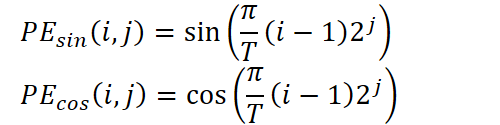
where T denotes the period of the corresponding component, i represents the time point, and j is the frequency index in the spectrum.

These vectors encode temporal dependencies across multiple scales, enabling the model to capture daily cycles, seasonal effects, and macroeconomic phases.

After this, they are concatenated with the normalized values of the time series. The resulting vector represents the embedding of the time point.

The sequence is then processed using a set of causal convolutional layers. Multiple parallel convolutions with unique windows allow capturing different time scales. Each convolution captures information at certain levels: from local fluctuations to long-term trends. Their outputs are merged into an enriched representation for every time step. This is particularly valuable for financial data, where a single candlestick may simultaneously represent a short-term market impulse and be a part of a broader market trend.

Next, the representation is projected into a higher-dimensional space, allowing the data to be prepared for entering the main model block. At this stage, a modified inception layer is connected, combining convolutional kernels of different sizes, integrating both local and global features. The resulting activation at each time step contains information from different levels of generalization while preserving output dimensionality and maintaining robustness to missing values and noise.

The core of the architecture consists of Mamba-based blocks, an innovative implementation of State Space Models (SSMs) with linear complexity in sequence length. Each block implements a generalized SSM structure in which the hidden state is updated using the matrices A, B, C, D, that are trained together with other model parameters:

Thus, each moment in time depends on both the previous state and the current input. This provides stable long-term memory and flexible adaptation to the current market context. Each such block is followed by Layer Normalization, which removes distributional bias and normalizes the activation distribution, resulting in more stable training. This is followed by an additional causal convolutional layer that supports information flow along the time axis.

The number of such blocks in a stack can vary depending on the desired depth of generalization. Lower layers specialize in capturing short-term market behavior, such as rapid pullbacks, momentum, and news-driven fluctuations. Higher layers gradually learn broader market cycles, seasonal dynamics, and recurring formations. The stack functions as a neural spectrum, with each layer responsible for a distinct temporal frequency range.

The final stage is the decoder. All activations are projected through a linear layer into one or more output channels. When uncertainty estimation is required, a dedicated prediction head is used to output the logarithm of the forecast variance:

For classification tasks, a Softmax prediction head produces probabilities of the analyzed classes.

One of Mamba4Cast's defining characteristics is its ability to perform Zero-Shot generalization. To achieve this, the authors introduce a unique pretraining stage based on an extensive synthetic dataset. This dataset includes time series generated from stochastic differential equations (SDEs), manually designed patterns (reversals, consolidations, and momentum impulses), as well as randomly generated rules.

The model is trained simultaneously using multiple loss functions: Mean Squared Error (MSE), Negative Log-Likelihood (NLL), and cross-entropy loss for regime-switch prediction. This allows the model to develop a robust, universal view of market patterns that can adapt to new assets and time scales.

Taken together, these characteristics make Mamba4Cast not just an experimental model, but provide a practical foundation for building predictive trading systems, market regime detection algorithms, and volatility forecasting solutions.

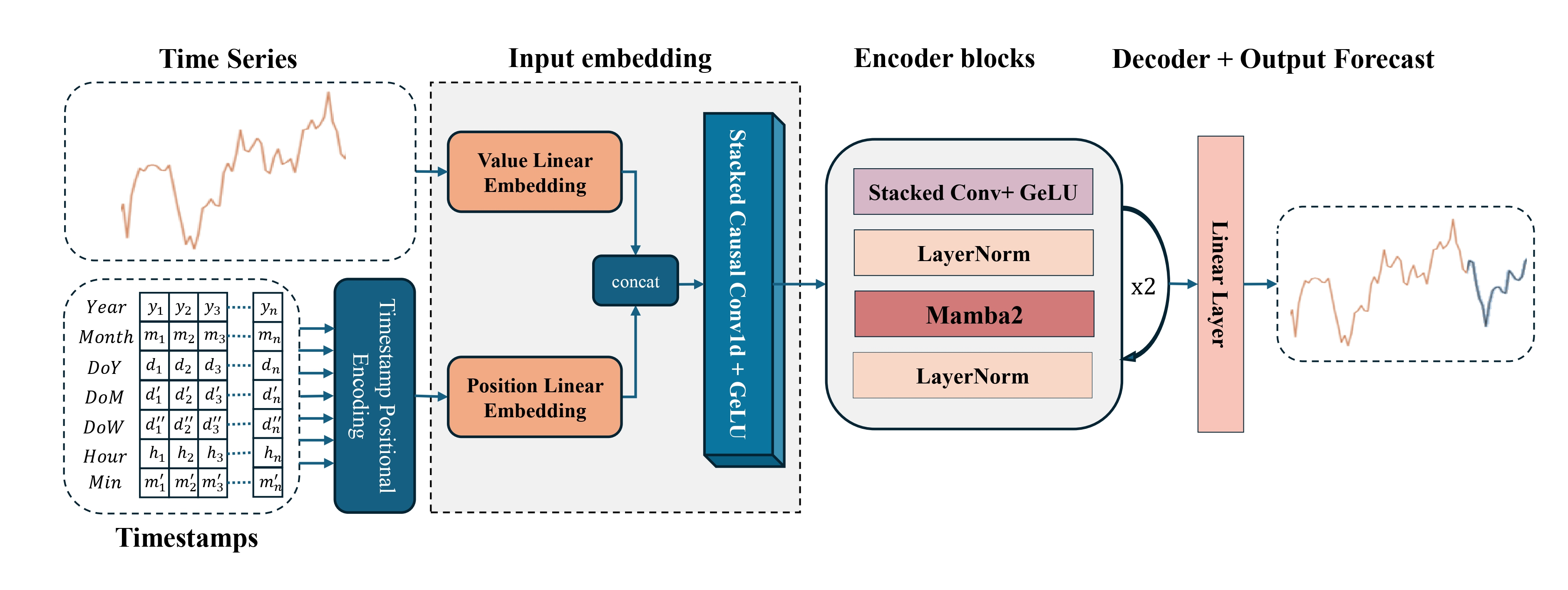
The authors' visualization of the Mamba4Cast framework is presented below.

Implementation in MQL5

Having explored the theoretical foundations of the Mamba4Cast architecture, we now move to the practical side — implementing its core components in MQL5. Our first task is to build the temporal positional encoding module, without which no modern forecasting model can correctly interpret the analyzed sequence as a genuine timeline.

Our library already includes several conventional positional embedding implementations, ranging from simple sinusoidal encodings to learnable tables. However, all of them treat a time series merely as an ordered sequence of elements, without considering the actual timestamps at which observations were recorded. The authors of Mamba4Cast insist that every time step should instead be encoded using its true temporal context: minute, hour, day of the week, day of the month, month, and even year — all of which influence market dynamics. According to their approach, an independent sinusoidal decomposition is constructed for each temporal component. So, our first practical block will be devoted to this deep time representation.

This stage fundamentally determines how the model perceives time: not simply as a sequence of bars, but as a stream of events at precisely defined moments. Without an accurate representation of timestamps, even the most sophisticated algorithm becomes meaningless, since markets react differently depending on the minute, hour, or day.

Temporal Encoding on the OpenCL Side

Rather than using the powerful but cumbersome approach of precomputed harmonic lookup tables, our implementation uses an OpenCL kernel to compute positional encodings directly from real timestamps in real time. This eliminates the need to store large sine and cosine tables in memory, avoids step-effects between adjacent points, and significantly simplifies the Expert Advisor logic.

In this approach, each time step enters the OpenCL kernel with two groups of information: its numerical features (price, volume, indicators) and its event timestamp. The timestamp is transformed into a vector that informs the model precisely when the event occurred: during the peak of a trading session or the quiet hours of a weekend, at the beginning of a month or on the eve of a new year.

The benefits of this approach are immediately apparent. First, it produces perfectly smooth positional encodings, ensuring that neighboring embeddings remain continuous without artificial jumps. Second, eliminating lookup tables results in less code, fewer synchronization issues, and reduced memory consumption in the platform. Thirdly, on-the-fly calculation makes embedding even more relevant: there's no need to rebuild tables when changing settings or periods — just change the period values, and the model instantly adapts to the new requirements.

The algorithm for adding temporal encodings into analyzed data on the OpenCL side implies surrounding each bar with its own harmonic vector describing the position within a cycle where it was formed. The TSPositionEncoder kernel receives pointers to three arrays:

• data with inputs,
• time with timestamps,
• period array defining the duration of each calendar cycle.

__kernel void TSPositonEncoder(__global const float2* __attribute__((aligned(8))) data,
                               __global const float* time,
                               __global float2* __attribute__((aligned(8))) output,
                               __global const float* period
                              )
  {
   const int id = get_global_id(0);
   const int freq = get_global_id(1);
   const int p = get_global_id(2);
   const int total = get_global_size(0);
   const int freqs = get_global_size(1);
   const int periods = get_global_size(2);

The kernel will be executed in a three-dimensional space:

• the length of the analyzed sequence (number of time steps),
• the number of harmonics for each period,
• the number of periods.

In the kernel body, each execution thread immediately determines its coordinates across all three dimensions.

First, for each time step (index id) and for each harmonic (freq) in the period (p), the core calculates a coordinate within a period: the real time is divided by the cycle length, turning the absolute value time[id] into the number of full periods. The fractional part is multiplied by π and the power of two 2^(freq+1). The resulting value val becomes the argument of the sine and cosine functions, where the first harmonic spans the entire cycle, the second divides it into halves, the third into quarters, and so forth.

   const int shift = id * freqs + freq;
   const float2 d = data[shift * periods + p];
   const float t = time[id] / period[p];
   float val = M_PI_F * t * pow(2.0f, freq + 1);

This value is then added to the source embedding. Each OpenCL thread loads the pair of values from data corresponding to the current time step, harmonic, and temporal cycle, adds sin(val) to the first element and cos(val) to the second. The resulting vector is saved to the output buffer. This operation enriches every point in the time series with additional features that precisely encode its position within calendar patterns.

   output[shift * periods + p] = (float2)(d.s0 + sin(val), d.s1 + cos(val));
  }

The advantage of this approach is that all computations are performed on the fly inside the GPU kernel, eliminating the need for large lookup tables or additional CPU-side processing. Any modifications — for example, adding a new temporal period or increasing the number of harmonics — require only adjustments to the dimensions of the three-dimensional grid and updates to the period array. At the same time, the representation remains perfectly continuous thanks to the smooth nature of sine and cosine functions, while GPU parallelism enables the simultaneous processing of large numbers of observations without delays.

As a result, every market event receives its own unique embedding that reflects not only its numerical characteristics, such as price or volume, but also the exact moment at which it occurred. This provides Mamba4Cast with a much richer temporal context, making its forecasting process genuinely time-aware.

Since the event timestamps in our implementation are not trainable parameters, only the feed-forward pass is required. Specifically, we need only compute the embedding vectors in the OpenCL kernel. There is no need to propagate gradients through the timestamps or update the timestamps themselves. This allows us to eliminate the backpropagation pass entirely, simplifying the architecture and reducing positional encoding to a purely deterministic function of time.

Temporal Encoding Object

On the main program side, the temporal encoding algorithms are implemented in the CNeuronTSPositionEncoder class, whose structure is presented below.

class CNeuronTSPositionEncoder   :  public CNeuronBaseOCL
  {
protected:
   CNeuronConvOCL             cProjection;
   CNeuronBatchNormOCL        cNorm;
   CBufferFloat               cPeriods;
   //---
   virtual bool               AddPE(CBufferFloat *time);
   //---
   virtual bool               feedForward(CNeuronBaseOCL *NeuronOCL) override { return false; }
   virtual bool               feedForward(CNeuronBaseOCL *NeuronOCL,
                                          CBufferFloat *SecondInput) override;
   virtual bool               updateInputWeights(CNeuronBaseOCL *NeuronOCL) override;
   virtual bool               calcInputGradients(CNeuronBaseOCL *NeuronOCL) override;

public:
                     CNeuronTSPositionEncoder(void) {};
                    ~CNeuronTSPositionEncoder(void) {};
   //---
   virtual bool               Init(uint numOutputs, uint myIndex, COpenCLMy *open_cl,
                                   uint window, uint units_count, uint &periods[], uint freqs,
                                   ENUM_OPTIMIZATION optimization_type, uint batch);
   //---
   virtual int                Type(void) override  const   {  return defNeuronTSPositionEncoder;   }
   //---
   virtual bool               Save(int const file_handle) override;
   virtual bool               Load(int const file_handle) override;
   //---
   virtual bool               WeightsUpdate(CNeuronBaseOCL *source, float tau) override;
   virtual void               SetOpenCL(COpenCLMy *obj) override;
   //---
   virtual uint               GetWindow(void) const { return cProjection.GetWindow(); }
   virtual uint               GetWindowOut(void) const { return cProjection.GetFilters(); }
   virtual uint               GetUnits(void) const { return cProjection.GetUnits(); }
  };

In the presented structure, three internal objects immediately stand out. At first glance, they may appear redundant given that temporal encoding is performed on the OpenCL side. However, these components are precisely responsible for ensuring that every analyzed data sequence is properly packaged and scaled before the temporal context is added.

First, cProjection receives arbitrary feature arrays coming from the previous layer of the neural network and transforms them into uniform vectors of a fixed dimensionality. Due to this, the remaining parts of the code do not have to bother about the number of input features and their internal organization — the output of cProjection always has a predictable structure, ready for batch normalization and positional encoding.

Second, cNorm serves as a stability mechanism. In practice, prices, volumes, and any stochastic signals may jump across value ranges. If sinusoidal and cosine values within the range [-1,1] were added immediately after projection, some information could be lost. To prevent this, the output of cProjection is passed through batch normalization, bringing the mean to zero and the variance to one. Only after this are the temporal harmonics introduced. This ordering ensures that temporal features become an organic extension of the processed data rather than an additional source of uncontrolled noise.

Finally, cPeriods stores the fixed set of temporal cycle periods.

This separation of responsibilities makes the class simultaneously flexible (it accepts arbitrary input data), robust (it always brings representations into a stable form), and precise (while preserving the absolute continuity of temporal encoding).

To transform the CNeuronTSPositionEncoder class from a declarative structure into a fully functional neural network component, all internal modules must be initialized correctly. This task is handled by the Init method.

bool CNeuronTSPositionEncoder::Init(uint numOutputs, uint myIndex, COpenCLMy *open_cl,
                                    uint window, uint units_count, uint &periods[], uint freqs,
                                    ENUM_OPTIMIZATION optimization_type, uint batch)
  {
   if(!CNeuronBaseOCL::Init(numOutputs, myIndex, open_cl, 2 * units_count * freqs * periods.Size(),
                                                                         optimization_type, batch))
      return false;

The method strictly follows the architectural logic described above: projection → normalization → temporal feature addition.

At the first step, we call the corresponding method of the parent class. It defines the general parameters of the object. Note that when specifying the output tensor size, the product of the received parameters is multiplied by 2. The reason is that each temporal harmonic is represented by two components: sine and cosine.

Next, the temporal cycle buffer is initialized. The periods are specified in seconds.

   cPeriods.BufferFree();
   if(!cPeriods.AssignArray(periods) ||
      !cPeriods.BufferCreate(OpenCL))
      return false;

Next, we initialize the input data projection layer into a fixed-dimensional space of: 2 × number of frequencies × number of periods. This size corresponds to the number of channels that will receive temporal information. Essentially, we configure the filters responsible for preparing each segment of the time series before temporal phases are added.

   int index = 0;
   if(!cProjection.Init(0, index, OpenCL, window, window, 2 * freqs * cPeriods.Total(), units_count,
                                                                           1, optimization, iBatch))
      return false;
   cProjection.SetActivationFunction(TANH);

The use of the TANH activation function during the projection stage is not merely a stylistic choice, it serves the practical purpose of constraining output amplitudes to the range [-1,1]. This provides several important advantages.

If the original data contains noise, jumps, or extreme values, TANH acts as a soft limiter, smoothing large deviations and making the model's behavior more stable. This is particularly important for financial time series, where unexpected candlesticks or volume spikes can disrupt the behavior of an entire neural network.

Additionally, TANH provides a smooth derivative across the entire input range, which is important during subsequent gradient propagation. This reduces the risk of neuron saturation and contributes to faster and more stable convergence.

Once the projection operation is complete, its output is passed to cNorm, where the mean values and scale are adjusted. This protects the temporal sine-cosine signals from being overwhelmed by excessively large amplitudes and ensures reliable temporal encoding.

   index++;
   if(!cNorm.Init(0, index, OpenCL, cProjection.Neurons(), iBatch, optimization))
      return false;
   cNorm.SetActivationFunction(None);

The final refinement is that, since temporal encoding is not a trainable component in the traditional sense, the general activation function is disabled and gradients are simply propagated from external interfaces to cNorm.

   SetActivationFunction(None);
   if(!SetGradient(cNorm.getGradient(), true))
      return false;
//---
   return true;
  } 

Moving on to the implementation of the feed-forward pass in the CNeuronTSPositionEncoder class, it should be emphasized that this stage represents the logical completion of the entire temporal encoding procedure. This is where the projected and normalized information from the original sequence is combined with the detailed temporal structure represented by harmonics calculated from the actual timestamps of incoming data.

The feedForward method carefully divides the process into three sequential stages. It should be noted that the method receives pointers to two separate data sources. The primary information stream contains the analyzed sequence, while the secondary stream contains the corresponding timestamps.

bool CNeuronTSPositionEncoder::feedForward(CNeuronBaseOCL *NeuronOCL, CBufferFloat *SecondInput)
  {
   if(!cProjection.FeedForward(NeuronOCL))
      return false;

First, the feed-forward pass of the input projection layer is executed. At this stage, input data of any dimensionality is transformed into the predefined number of features, ensuring dimensional compatibility for adding the required number of temporal harmonics.

The resulting projections are then passed through the normalization layer.

   if(!cNorm.FeedForward(cProjection.AsObject()))
      return false;

The purpose of normalization is to smooth statistical differences between the features of the analyzed data and prepare them for combination with the temporal harmonics.

Finally, the last stage calls the wrapper method for the previously described temporal encoding kernel. In real time, this kernel calculates sine-cosine harmonics for every time step and every specified frequency based on the current timestamp value and the set of periods.

   return AddPE(SecondInput);
  }

This operation does not depend on trainable parameters and does not require gradient propagation, because time represents an external deterministic factor.

As a result, the output is a rich representation combining both meaningful characteristics of the input data and the precise temporal context in which those observations occurred — not according to their sequential index, but according to the actual rhythm of events.

The backpropagation processes in the CNeuronTSPositionEncoder class are deliberately concise in structure while remaining essential. All computations follow the standard approach of propagating error gradients back to the original input data. The main computational flow passes through two key components: the projection layer (cProjection) and the normalization layer (cNorm). Each of these contains trainable parameters and therefore requires optimization.

In practice, this means that when the updateInputWeights and calcInputGradients methods are called, our object simply delegates execution sequentially to the corresponding methods of its internal components.

This approach ensures modularity and repeatability of the logic: changes in the optimization mechanism of an individual layer automatically propagate throughout the entire system without requiring modifications to higher-level code. This is especially important for scalable neural network architectures.

However, one important point should be emphasized. Although the feedForward method receives two information streams — the primary input sequence and the timestamp array — only the primary information stream participates in backpropagation. This is entirely justified.

The reason is that temporal encoding in CNeuronTSPositionEncoder contains no trainable parameters. It represents a fixed, deterministic transformation applied to timestamps. Moreover, we intentionally do not propagate error gradients back to the timestamp level. These values are external to the model and should not be modified during optimization.

This design philosophy makes the architecture not only clean and stable but also logically consistent: temporal information is used for contextualization, not for training.

The complete source code of this class and all its methods is provided in the attachment.

We have now reached the reasonable boundaries of this article format. We have analyzed the fundamental components of temporal encoding, implemented key concepts, and presented the layer architecture in code in a clear and structured form. However, as the saying goes, not everything can be done at once.

Our implementation is not yet complete. A significant amount of work remains ahead, requiring a careful and thoughtful approach. We will take a short pause and continue in the next article.

Conclusion

In this article, we explored the Mamba4Cast framework, designed to address one of the fundamental challenges in time-series analysis: building a flexible and scalable model capable of capturing the complex structure of dynamic temporal data. We examined how the authors overcame the traditional limitations of classical models by integrating modern architectural approaches, including State Space Models (SSMs) enhanced with Causal Convolution mechanisms, and complementing them with precise positional encoding based on real-world timestamps.

As we gradually explored the framework's structure, we analyzed in detail the process of constructing temporal features. We demonstrated how simple yet powerful harmonic functions can transform raw timestamps into meaningful embeddings that reflect the cyclical nature of market dynamics. Using the OpenCL implementation as an example, we examined how such embeddings can be generated efficiently directly within the computational kernel, without additional lookup tables or processing delays.

However, our work is not yet complete. In the next article, we will continue this research and demonstrate how temporal embeddings interact with the architectural blocks of the model, preserving the integrity of the analysis and improving forecasting accuracy.

References

• Mamba4Cast: Efficient Zero-Shot Time Series Forecasting with State Space Models
• Other articles from this series

Programs Used in the Article

#	Name	Type	Description
1	Research.mq5	Expert Advisor	Expert Advisor for collecting samples
2	ResearchRealORL.mq5	Expert Advisor	Expert Advisor for collecting samples using the Real-ORL method
3	Study.mq5	Expert Advisor	Expert Advisor for offline model training
4	StudyOnline.mq5	Expert Advisor	Expert Advisor for online model training
4	Test.mq5	Expert Advisor	Expert Advisor for model testing
5	Trajectory.mqh	Class library	System state and model architecture description structure
6	NeuroNet.mqh	Class library	A library of classes for creating a neural network
7	NeuroNet.cl	Code library	OpenCL program code