

Neural Networks in Trading: Generalizing Time Series Without Data-Specific Dependence (Core Model Modules)
 934
934
 0
0

Introduction
In the previous article, we introduced the Mamba4Cast framework and its core components: the SSM module and the Prior-data Fitted Networks (PFNs) mechanism. This framework establishes a solid foundation for time-series forecasting and have the potential to become a powerful addition to a trader's analytical toolkit.
Mamba4Cast was designed not for lengthy warm-up on every new time series, but for immediate deployment. Thanks to the concept of Zero-Shot Forecasting, the model can produce high-quality forecasts on real-world data without additional training or hyperparameter tuning. As a result, traders no longer need to spend days searching for the optimal configuration.
The model's high execution speed is rooted in the linear computational complexity of its SSM modules. Unlike transformer architectures, whose computational cost grows quadratically with sequence length, each processing step in Mamba4Cast is executed in constant time. This enables near-instant inference even on very long sequences while maintaining minimal latency. In trading, where execution speed can determine the outcome of a trade, this advantage is difficult to overstate.
In addition, Mamba4Cast generates the entire forecast horizon at once rather than producing it one step at a time. This design avoids the accumulation of errors typical of autoregressive models and delivers more stable future trajectories. Trading strategies receive a complete outlook immediately, enabling more confident and informed decision-making.
Equally significant is the training methodology based on synthetic scenarios. The model was trained on millions of artificially generated time series. This allows Mamba4Cast to develop a generalized intuition and operate reliably across a wide range of conditions. This approach improves robustness to noise and abrupt market changes. Consequently, this reduces the likelihood of unexpected failures in production environments.
Despite the power of its underlying mechanisms, Mamba4Cast remains computationally efficient. According to experiments conducted by the framework's authors, it achieves accuracy comparable to modern transformer-based foundation models while requiring substantially fewer computational resources. This makes it practical even on resource-constrained infrastructure and suitable for direct integration into trading terminals without the need for high-end GPU clusters.
It is precisely this combination of instant deployment, exceptional inference speed, holistic forecasting, robustness to noisy data, and computational efficiency that makes Mamba4Cast a genuinely groundbreaking framework for time-series forecasting.
The authors' visualization of the >Mamba4Cast framework is presented below.
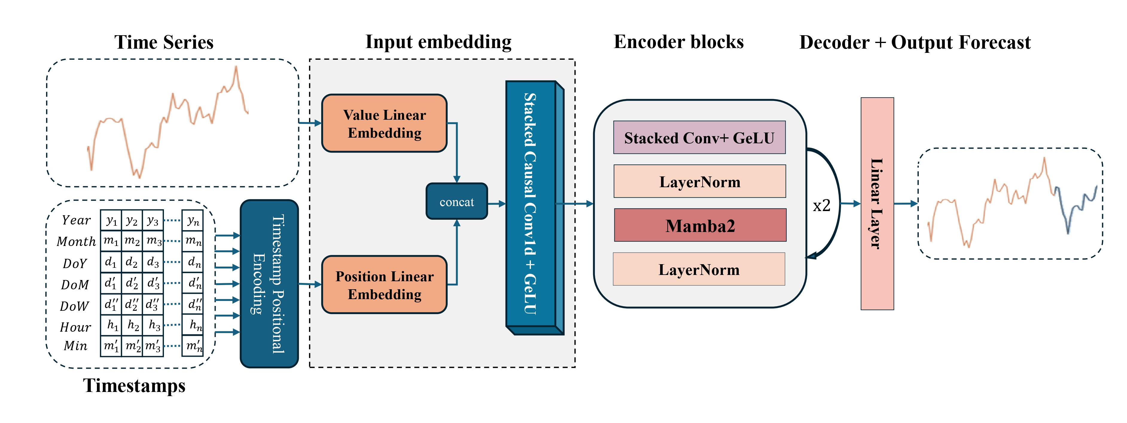
In the practical section of the previous article, we concluded by implementing the temporal encoding object — a key component responsible for providing positional representations of the input data within the time sequence. This component completed the model's initialization pipeline and became an essential part of the architectural preparation of the input signal. Without it, the framework would be unable to correctly capture temporal dependencies.
Today, we will continue from that point.
Data Preprocessing Module
The development logic is straightforward: before performing any computations, forecasting price movements, or generating trading signals, the input data must first be prepared properly. As with any machine learning system, the performance of Mamba4Cast depends directly on the quality of the incoming data stream. If the model receives noisy inputs, inconsistent scales, or fragmented structures, even the most advanced architecture cannot compensate. For this reason, our focus is now on the data preprocessing module.
This module is far more than an auxiliary stage. It serves as the bridge between raw market data and the structured inputs that the model can effectively interpret. This stage performs normalization, scaling, window construction, mask generation, and — most importantly — data contextualization through additional feature channels. Together, these operations prepare the information for processing by the core model and establish the foundation for all subsequent forecasting.
Our objective is not merely to load price quotes and indicator values. We must transform them into a unified scale, identify the boundaries of valid windows, generate masks for unavailable values, and synchronize all feature channels in time. Only after these steps can we pass the data to the Encoder and expect that it will be interpreted correctly.
In the practical section of the previous article, we completed the implementation of the temporal encoding object — one of the key components of data preprocessing and an important element of the Mamba4Cast architecture. This component enables the model to perceive a sequence of market events not as an abstract collection of numbers, but as structured information with a well-defined order and temporal rhythm.
To implement this approach, we will develop a specialized class CMamba4CastEmbedding, which occupies a central role within the preprocessing stage. Its structure is presented below.
class CMamba4CastEmbeding :   public CNeuronBaseOCL
  {
protected:
   CNeuronConvOCL             cProjection;
   CNeuronBatchNormOCL        cNorm;
   CNeuronTSPositionEncoder   cProjectionWithTE;
   //---
   virtual bool               feedForward(CNeuronBaseOCL *NeuronOCL) override { return false; }
   virtual bool               feedForward(CNeuronBaseOCL *NeuronOCL, CBufferFloat *SecondInput) override;
   virtual bool               updateInputWeights(CNeuronBaseOCL *NeuronOCL) override;
   virtual bool               calcInputGradients(CNeuronBaseOCL *NeuronOCL) override;

public:
                     CMamba4CastEmbeding(void) {};
                    ~CMamba4CastEmbeding(void) {};
   //---
   virtual bool               Init(uint numOutputs, uint myIndex, COpenCLMy *open_cl,
                                   uint window, uint window_out, uint units_count, uint &periods[],
                                   ENUM_OPTIMIZATION optimization_type, uint batch);
   //---
   virtual int                Type(void) override  const   {  return defMamba4CastEmbeding;   }
   //---
   virtual bool               Save(int const file_handle) override;
   virtual bool               Load(int const file_handle) override;
   //---
   virtual bool               WeightsUpdate(CNeuronBaseOCL *source, float tau) override;
   virtual void               SetOpenCL(COpenCLMy *obj) override;
  };
The core idea is to transform the stream of initial information into a structured and information-rich representation suitable for the subsequent forecasting stages. To achieve this, the class follows a modular design, combining several specialized modules, each responsible for a specific data transformation.
It is worth noting that all internal objects of the CMamba4CastEmbedding class are declared statically. Consequently, both the constructor and destructor remain empty because no dynamic memory management is required — the objects are created and destroyed automatically. This architectural decision simplifies object lifecycle management, minimizes the risk of memory leaks, and eliminates potential errors associated with dynamic memory allocation, which is particularly important in high-performance trading systems.
Initialization of all internal modules is performed in the Init method, whose parameters define the main characteristics of the object being created.
bool CMamba4CastEmbeding::Init(uint numOutputs, uint myIndex, COpenCLMy *open_cl,
                               uint window, uint window_out, uint units_count, uint &periods[],
                               ENUM_OPTIMIZATION optimization_type, uint batch)
  {
   if(periods.Size() <= 0)
      return false;
   int freqs = (int(window_out / 2 + 2 * periods.Size()) - 1) / int(2 * periods.Size());
   if(freqs <= 0)
      return false;
The method begins by verifying that the array of analyzed time-series periods contains data. This validation is necessary because temporal encoding requires at least one period to compute correctly. Immediately afterward, the method calculates the freqs parameter, which specifies the number of frequency harmonics assigned to each period.
The logic behind this parameter deserves a more detailed explanation. One of the initialization parameters (window_out) defines the embedding dimension for a single time step. As discussed previously, each temporal slice of data must be represented in two complementary forms: first, as a pure value independent of time, and second, in combination with temporal features encoded through harmonic components. The final embedding combines both representations within a single vector. But we have only one amount of memory allocated for this representation. Therefore, only half of the user-defined embedding size can be used for temporal encoding. The remaining half is reserved for the standard projection of the input data.
Now let's consider how this temporal half is distributed among the frequency components. The authors of Mamba4Cast used an approach similar to the positional encoding used in transformer architectures: for every specified period, both sine and cosine functions are generated to describe the phase and frequency of oscillations. Consequently, each frequency component requires two harmonic functions — a sine and a cosine. Therefore, the total number of frequency components must be at least twice the number of periods specified in the input array.
To avoid confusion, we use a straightforward formula which however requires careful attention: we divide half of window_out by twice the number of specified periods. The resulting value determines how many frequency components can be allocated to each period. This value must always be greater than zero. Otherwise, the model would be unable to generate even a single harmonic pair, making temporal encoding impossible.
In practice, this means that when selecting the embedding size for a single time step, the objective should not simply be to increase model capacity, but to ensure that every analyzed period is represented by at least one harmonic pair.
We then calls the corresponding initialization method of the parent class, where all inherited objects and interfaces are initialized.
if(!CNeuronBaseOCL::Init(numOutputs, myIndex, open_cl, window_out * units_count, optimization_type, batch))
   return false;
After its successful execution, we proceed to the sequential initialization of the internal modules of our class. The first component is cProjection, the convolutional projection layer responsible for mapping the input data into a compact representation.
int index = 0;
if(!cProjection.Init(0, index, OpenCL, window, window, window_out - 2 * freqs * periods.Size(), units_count,
                                                                                   1, optimization, iBatch))
   return false;
cProjection.SetActivationFunction(TANH);
This module generates embeddings of the original data without incorporating temporal information. We use the TANH activation function to introduce nonlinearity, allowing the network to emphasize meaningful patterns hidden within the raw numerical data while reducing the influence of outliers.
The batch normalization layer (cNorm) subsequently adjusts these projected features, eliminating distributional bias and improving computation stability.
index++;
if(!cNorm.Init(0, index, OpenCL, cProjection.Neurons(), iBatch, optimization))
   return false;
cNorm.SetActivationFunction(None);
Generation of embeddings enriched with temporal information is handled by the temporal encoding module (cProjectionWithTE), which is particularly important for capturing seasonal trends and dynamic changes in market behavior.
   index++;
   if(!cProjectionWithTE.Init(0, index, OpenCL, window, units_count, periods, freqs, optimization, iBatch))
      return false;
   SetActivationFunction(None);
//---
   return true;
  }
In the framework logic, this sequential initialization process guarantees that each submodule receives a consistent and compatible configuration, enabling the efficient integration of temporal information with the original input data.
One of the key stages of the CMamba4CastEmbedding module is the execution of the feedForward method, which performs the forward propagation of data through every component of the preprocessing architecture. It is at this stage that the foundation is established for the subsequent modules, allowing them to operate not on raw inputs, but on carefully prepared representations that already incorporate both the structural characteristics of the original signal and its temporal context.
bool CMamba4CastEmbeding::feedForward(CNeuronBaseOCL *NeuronOCL, CBufferFloat *SecondInput)
  {
   if(!cProjection.FeedForward(NeuronOCL))
      return false;
The process begins by passing the input data to cProjection. This compact convolutional block projects the original signal into a latent feature space. This step enables the system to focus immediately on the most informative patterns and significant changes in the input stream.
The extracted features are then passed to cNorm. This normalization layer is responsible for scaling the activations to a stable range while eliminating spikes, outliers, and distributional shifts.
if(!cNorm.FeedForward(cProjection.AsObject()))
   return false;
Without normalization, deep neural architectures often suffer from exploding or vanishing gradients. Here, normalization acts as a stabilizing mechanism, promoting consistent model behavior during both training and inference.
However, the distinctive feature of the Mamba4Cast architecture lies in its second processing path. In parallel, the original input data is forwarded to cProjectionWithTE, the module responsible for temporal encoding.
if(!cProjectionWithTE.FeedForward(NeuronOCL, SecondInput))
   return false;
Unlike the initial projection stage, which relies solely on convolutional operations, this module also receives a secondary input SecondInput. Through this channel, precomputed temporal markers for every time step are introduced into the computation. This enables the module not only to analyze feature values themselves, but also to interpret them within their precise temporal context, improving the model's sensitivity to seasonal, cyclical, and phase-related market dynamics.
The final stage of the process is the fusion operation. The representations generated by the two processing paths are concatenated into a single tensor.
   if(!Concat(cNorm.getOutput(), cProjectionWithTE.getOutput(), Output, cProjection.GetFilters(),
              cProjectionWithTE.GetWindowOut(), cProjection.GetUnits()))
      return false;
//---
   return true;
  }
The resulting output is a dense, multi-level representation of every time step that combines both the original feature information and an enriched temporal structure. It is this comprehensive representation of the time sequence that serves as the foundation for all subsequent operations performed by the model.
As is well known, forward propagation alone is not enough to train a neural network. For the model to adapt to the data, it must also perform correct error backpropagation. This part is performed by the calcInputGradients method. In essence, it serves as the model's internal error analysis mechanism, activated after a prediction has been generated to determine where errors occurred and how the model parameters should be adjusted.
bool CMamba4CastEmbeding::calcInputGradients(CNeuronBaseOCL *NeuronOCL)
  {
   if(!NeuronOCL)
      return false;
The method first checks what object is involved. It is important to ensure that every component used in gradient computations has been initialized correctly. Afteк this check, execution proceeds to the DeConcat method, which separates the previously concatenated gradient vector into two independent information streams.
if(!DeConcat(cNorm.getGradient(), cProjectionWithTE.getGradient(), Gradient, cProjection.GetFilters(),
             cProjectionWithTE.GetWindowOut(), cProjection.GetUnits()))
   return false;
Recall that during the feed-forward pass, the normalized feature representation and the temporal embeddings were merged into a single tensor. During backpropagation, however, these streams must be separated again so that each processing branch can be trained independently.
After the gradients have been separated, the main backpropagation process begins, propagating the error gradients through both information streams back to the original input data. First, we perform operations with the branch that does not contain temporal information.
if(!cProjection.calcHiddenGradients(cNorm.AsObject()))
   return false;
if(!NeuronOCL.calcHiddenGradients(cProjection.AsObject()))
   return false;
The computation proceeds to the temporal context branch. Before propagating the gradients, however, it is necessary to preserve the previously computed data. For this, the method temporarily redirects the pointer to the gradient buffer associated with the original input object. After that, the gradient computations are performed.
   CBufferFloat *temp = NeuronOCL.getGradient();
   if(!NeuronOCL.SetGradient(NeuronOCL.getPrevOutput(), false) ||
      !NeuronOCL.calcHiddenGradients(cProjectionWithTE.AsObject()) ||
      !SumAndNormilize(temp, NeuronOCL.getGradient(), temp, cProjection.GetWindow(), false, 0, 0, 0, 1) ||
      !NeuronOCL.SetGradient(temp, false)
     )
      return false;
//---
   return true;
  }
The final step consists of summing the gradients from both information streams. After that, all buffer pointers are restored to their original state, and the method terminates by returning a the Boolean result of the operation to the calling program.
The result of this carefully designed procedure is the correct distribution of error gradients throughout the module, ensuring balanced weight updates.
Optimization of the trainable parameters in each submodule is performed by the updateInputWeights method. Weight updates are performed by sequentially calling the corresponding update methods of internal objects. This step-by-step procedure reflects the principle of isolated weight management, providing fine-grained control over the training process and allowing changes to be made independently of the overall system architecture. If any stage of the update process fails, the method immediately returns an error, thereby preserving the consistency of the model's state.
The updateInputWeights method code is available in the attachments to the article. They also contain the full code of the CMamba4CastEmbedding class and all of its methods.
In summary, the CMamba4CastEmbedding class is far more than a collection of data transformation algorithms. It is a carefully engineered module in which every function is tightly integrated with the overall logic of the Mamba4Cast framework. It provides high-quality preprocessing of the input data, enabling the model to extract meaningful features efficiently, capture temporal dynamics, and learn effectively through properly propagated error gradients.
Encoder
The next stage of our implementation is the construction of the Encoder proposed by the authors of the Mamba4Cast framework. This component plays a crucial role in extracting and structuring features for subsequent forecasting. Its architecture is built around a stack of convolutional layers with different kernel sizes. Each convolutional layer focuses on capturing specific characteristics of the input data, after which their outputs are concatenated and normalized before being passed to the Mamba module. The number of repetitions of this block determines the depth of feature extraction, allowing the framework to adapt to tasks of varying complexity.
Of particular interest here is the stack of convolutional layers. A convolutional layer object has long been available in our library, and its use presents no difficulties. However, in the conventional approach, each convolutional layer is instantiated as a separate object and processed sequentially. When convolution kernels of different sizes are used, the number of such objects grows significantly, while sequential execution substantially increases the computational complexity of the model and, consequently, the training time.
To address this limitation, we designed a dedicated object capable of processing multiple convolutional layers in parallel. Such an object can launch computations simultaneously across multiple execution streams, dramatically reducing execution time. Internally, it distributes the workload by feeding the same input signal to several convolutional filters with different kernel sizes, then concatenating their outputs into a single tensor. This approach not only reduces the number of intermediate objects, but also makes considerably more efficient use of computational resources, particularly when executing on modern multi-threaded GPUs.
The concept itself is not entirely new. Previously, we implemented the CNeuronMultiWindowsConvOCL class, which supported convolutional operations with different kernel sizes. However, its design assumed a separate input buffer for each convolution window. In the present case, we face a different challenge: the same input stream must be processed using multiple convolution windows simultaneously.
The difficulty lies in the fact that changing the kernel size also changes the number of possible convolution operations. As the convolution window becomes larger, the number of positions where convolution can be applied decreases. Consequently, the computational workloads associated with different kernel sizes become unbalanced. This makes efficient parallel execution more difficult.
To solve this problem, we adopted zero padding, adding zeros to both the beginning and the end of the input vector. This technique extends the vector so that, regardless of convolution window size, the same number of operation threads can be used. As a result, the number of convolution operations is determined solely by the convolution stride, which remains identical for all kernel sizes. This equalizes the workload across parallel threads and greatly simplifies parallel processing.
The core logic on the OpenCL side implementation resides in a compact yet powerful FeedForwardMultWinConvWPad kernel, which simultaneously processes the same input stream through multiple convolution windows of different lengths.
__kernel void FeedForwardMultWinConvWPad(__global const float *matrix_w,
                                         __global const float *matrix_i,
                                         __global float *matrix_o,
                                         __global const int *windows_in,
                                         const int inputs,
                                         const int step,
                                         const int window_out,
                                         const int activation
                                        )
  {
   const size_t id = get_global_id(0);
   const size_t id_w = get_global_id(1);
   const size_t v = get_global_id(2);
   const size_t outputs = get_global_size(0);
   const size_t windows_total = get_global_size(1);
Each execution thread is identified by three coordinates:
- id — the index of the output tensor element;
- id_w — the convolution window index;
- v — the identifier of the univariate input stream.
This organization allows multiple convolution windows, positions, and input sequences to be processed in parallel using different operation parameters.
In the first step, the kernel determines the length of the current convolution window window_in, by retrieving it from the windows_in array using the current window identifier.
int window_in = windows_in[id_w];
Next, it computes the starting offset of the convolution window in the input buffer according to the current output tensor index. The offset is calculated so that the center of the convolution window aligns with position id. Since window sizes vary, the expression (window_in + 1) / 2 is used to ensure proper center alignment.
int window_in = windows_in[id_w];
int mid_win = (window_in + 1) / 2;
int shift_in = id * step - mid_win;
int shift_in_var = v * inputs;
The variable shift_in_var is then used to address the appropriate input sequence within the global input buffer.
The next step computes shift_weight, the offset in the global array of trainable parameters. Because the weights for each convolution window are stored consecutively taking into account their length and the bias coefficient, it is necessary to sum the sizes of all weight blocks preceding the current window id_w. This allows us to determine exactly where the weights for the current convolution start.
int shift_weight = 0;
for(int w = 0; w < id_w; w++)
   shift_weight += (windows_in[w] + 1) * window_out;
A nested loop is then launched over each output channel w_out, representing the embedding dimension in the result buffer generated after the convolution.
   for(int w_out = 0; w_out < window_out; w_out++)
     {
      float sum = matrix_w[shift_weight + window_in];
      //---
      for(int w = 0; w < window_in; w++)
         if((shift_in + w) >= 0 && (shift_in + w) < inputs)
            sum += IsNaNOrInf(matrix_i[shift_in_var + shift_in + w] * matrix_w[shift_weight + w], 0);
      //---
      int shift_out = (v * outputs + id) * window_out + w_out;
      matrix_o[shift_out] = Activation(sum, activation);
      shift_weight += window_in + 1;
     }
  }
For every output channel, the variable sum is initialized, which first takes the bias value (the final element of the weight block). The products of the input values and their corresponding weights are then added to that value. During this process, the algorithm explicitly checks whether the current input index falls outside the valid input range. If it does, the operation is skipped, which is equivalent to applying zero padding.
Once a lopp through the window has been completed, the result is processed by the activation function. The activation type is specified by the activation parameter, while the activation function is applied through the helper wrapper Activation. The final value is then written to the global output buffer matrix_o, taking all required offsets into account.
Finally, the shift_weight pointer advances by the size of the current window plus one additional element for the bias, positioning it at the weights of the next filter. Thus, each execution thread sequentially processes all output channels while computations remain fully parallel across all convolution windows and all input sequences.
The resulting algorithm is not only flexible but also exceptionally efficient. Convolutions at multiple scales are applied to the data simultaneously, providing a comprehensive multi-scale representation of the input. Zero padding eliminates the need for manual sequence trimming or post-processing to align embedding dimensions. Everything is performed dynamically during GPU execution.
This implementation demonstrates an important design principle: high performance is achieved not by simplifying the algorithm, but by carefully partitioning the computation, exploiting parallel execution, and precisely orchestrating every stage of the data transformation pipeline.
The next major stage is the computation of error gradients with respect to the original input data. Unlike the forward pass, this stage presents a considerably more challenging problem. Rather than simply applying a set of filters, we must propagate the contribution of every filter backward to reconstruct the gradient at the input level while correctly handling offsets and preserving tensor consistency.
This algorithm is implemented in the OpenCL kernel CalcHiddenGradientMultWinConvWPad. Its purpose is to aggregate error gradients across convolution windows of different lengths and across all output channels. In other words, it reconstructs the error propagated back to the original input sequence while accounting for both the activation nonlinearity and the convolutional filter structure.
__kernel void CalcHiddenGradientMultWinConvWPad(__global const float *matrix_w,
                                                __global const float *matrix_i,
                                                __global float *matrix_ig,
                                                __global const float *matrix_og,
                                                __global const int *windows_in,
                                                const int outputs,
                                                const int step,
                                                const int window_out,
                                                const int activation
                                               )
  {
   const size_t id_x = get_global_id(0);
   const size_t id_loc = get_local_id(1);
   const size_t id_win = id_loc / window_out;
   const size_t id_f = id_loc % window_out;
   const size_t v = get_global_id(2);
   const size_t inputs = get_global_size(0);
   const size_t size_loc = get_local_size(1);
   const size_t windows_total = size_loc / window_out;
Each thread within the kernel computes one element of the input-level gradient:
- id_x — the index of the position within the input sequence;
- id_loc — the local work-group identifier, which is decomposed into id_win (window index) and id_f (filter index within the output buffer);
- v — the identifier of the input sequence.
The first step computes shift_weight, which determines the exact starting position of the weight block corresponding to the current convolution window and channel. As before, the algorithm iterates through all preceding windows, accumulating their sizes until it reaches the correct position within the global weight array matrix_w.
   __local float temp[LOCAL_ARRAY_SIZE];
   const uint ls = min((uint)size_loc, (uint)LOCAL_ARRAY_SIZE);
//---
   int window_in = windows_in[id_win];
   int shift_weight = id_f * (window_in + 1);
   for(int w = 0; w < id_win; w++)
      shift_weight += (windows_in[w] + 1) * window_out;
Next, it determines the region of the output buffer in which the current input element could have participated — shift_out. This value is bounded below by zero and represents the earliest possible output position whose convolution window could still include the current input element id_x.
int shift_out = max((int)((id_x - window_in) / step), 0);
But this is not enough — then a cycle starts through all possible outputs out, in which our element could participate in a feed-forward pass.
float grad = 0;
int mid_win = (window_in + 1) / 2;
for(int out = shift_out; out < outputs; out++)
  {
   int shift_in = out * step - mid_win;
   if(shift_in > id_x)
      break;
   int shift_w = id_x - shift_in;
   if(shift_w >= window_in)
      continue;
   int shift_g = ((v * outputs + out) * windows_total + id_win) * window_out + id_f;
   grad += IsNaNOrInf(matrix_w[shift_w + shift_weight] * matrix_og[shift_g], 0);
  }
At each iteration, the kernel checks whether id_x belongs to the current convolution window. If it does, it computes the local offset shift_w within the window together with the corresponding output-gradient position shift_g. Multiplying the appropriate filter weight by the output gradient matrix_og yields that convolution's contribution to the input gradient. These contributions are accumulated into the variable grad.
At this point, each execution thread holds only a partial gradient. However, multiple threads within the same work-group may correspond to the same input position id_x while processing different filters or output channels. Therefore, an intermediate array is introduced in local memory - temp, and the summation cycle with synchronization barriers is started. Each thread first stores its partial result in temp.
for(int i = 0; i < size_loc; i += ls)
  {
   if(i <= id_loc && (i + ls) > id_loc)
      temp[id_loc % ls] = (i == 0 ? 0 : temp[id_loc % ls]) + grad;
   barrier(CLK_LOCAL_MEM_FENCE);
  }
Then, using parallel reduction folding, the array is summed in powers of two, leaving the final gradient across all channels and windows in temp[0].
uint count = ls;
do
  {
   count = (count + 1) / 2;
   if(id_loc < count && (id_loc + count) < ls)
     {
      temp[id_loc] += temp[id_loc + count];
      temp[id_loc + count] = 0;
     }
   barrier(CLK_LOCAL_MEM_FENCE);
  }
while(count > 1);
Finally, only the thread with id_loc == 0 writes the resulting gradient into the global input-gradient buffer matrix_ig. Before doing so, it invokes the Deactivation function, which applies the derivative of the activation function to the corresponding input value matrix_i. This step is essential: the gradient must be corrected according to the activation function; otherwise, the learning process would become incorrect.
 if(id_loc == 0)
    matrix_ig[v * inputs + id_x] = Deactivation(temp[0], matrix_i[v * inputs + id_x], activation);
}
This is one of the most computationally demanding stages of backpropagation. By dividing calculations into windows and channels, as well as using local memory, high efficiency is achieved even with a large number of parameters. Combined with the feed-forward pass, this step makes our algorithm not only modular and scalable, but also capable of handling very complex dependencies in financial time series without losing accuracy or performance.
The final step in this convolutional symphony is weight optimization. At this stage, the computed gradients are transformed into actual parameter updates. This is accomplished using the Adam optimization algorithm, extended to account for convolution windows of different sizes and zero padding. All of this logic is encapsulated in the UpdateWeightsMultWinConvAdamWPad kernel.
__kernel void UpdateWeightsMultWinConvAdamWPad(__global float *matrix_w,
                                               __global const float *matrix_og,
                                               __global const float *matrix_i,
                                               __global float *matrix_m,
                                               __global float *matrix_v,
                                               __global const int *windows_in,
                                               const int windows_total,
                                               const int window_out,
                                               const int inputs,
                                               const int step,
                                               const int outputs,
                                               const float l,
                                               const float b1,
                                               const float b2
                                              )
  {
   const size_t i = get_global_id(0);  // weight shift
   const size_t v = get_local_id(1);   // variable
   const size_t variables = get_local_size(1);
Each thread in this kernel is responsible for updating one specific parameter i — whether it is a filter coefficient or a bias. The variable v identifies the input sequence, while variables specifies the total number of sequences. Together, they allow gradients to be accumulated across all input sequences, resulting in more stable parameter updates.
At the beginning of execution, each thread determines which filter, output channel, and specific weight correspond to its parameter index i. This is accomplished by iterating over all convolution windows while maintaining the cumulative offset shift_before, which tracks the position of each window within the linear array of trainable parameters.
   __local float temp[LOCAL_ARRAY_SIZE];
   const uint ls = min((uint)variables, (uint)LOCAL_ARRAY_SIZE);
//---
   int step_out = window_out * windows_total;
//---
   int shift_before = 0;
   int window = 0;
   int number_w = 0;
   for(int w = 0; w < windows_total; w++)
     {
      int win = windows_in[w];
      if(shift_before <= i &&
         (win + 1)*window_out > (i - shift_before))
        {
         window = win;
         number_w = w;
        }
      else
         shift_before += (win + 1) * window_out;
     }
Once the window corresponding to i has been identified, we determine:
- window — the filter size width;
- number_w — window index;
- id_f — filter index;
- shift_in — offset relative to the beginning of the window (if it is equal to the window size, then it is bias);
- bias — a logical flag that determines whether the element being analyzed is a bias parameter.
int shift_in = (i - shift_before) % (window + 1);
int shift_in_var = v * inputs;
bool bias = (shift_in == window);
int mid_win = (window + 1) / 2;
int id_f = (i - shift_before) / (window + 1);
int shift_out = number_w * window_out + id_f;
int shift_out_var = v * outputs * step_out;
For ordinary filter coefficients, the kernel iterates over every out output position. At each position, it verifies that the corresponding input element lies within the valid input range. If so, it performs the standard gradient computation by multiplying the output gradient matrix_og by the corresponding input activation matrix_i, accumulating the products into grad.
float grad = 0;
if(!bias)
  {
   for(int out = 0; out < outputs; out++)
     {
      int in = out * step - mid_win + shift_in;
      if(in >= inputs)
         break;
      if(in < 0)
         continue;
      //---
      grad += IsNaNOrInf(matrix_og[shift_out_var + shift_out + out * step_out] * matrix_i[shift_in_var + in], 0);
     }
  }
else
  {
   for(int out = 0; out < outputs; out++)
      grad += IsNaNOrInf(matrix_og[shift_out_var + shift_out + out * step_out], 0);
  }
For bias parameters, the input activations are not required. Instead, the kernel simply accumulates the output gradients across all positions.
The next stage again employs local accumulation through the temp array. Its purpose is to aggregate gradients across all input sequences while reducing the influence of individual outliers. As before, a parallel reduction tree combined with synchronization barriers is used to perform the summation efficiently within each work-group. Only the thread with v == 0 (the first one) performs the final weight update.
//--- sum
   for(int s = 0; s < (int)variables; s += ls)
     {
      if(v >= s && v < (s + ls))
         temp[v % ls] = (s == 0 ? 0 : temp[v % ls]) + grad;
      barrier(CLK_LOCAL_MEM_FENCE);
     }
//---
   uint count = ls;
   do
     {
      count = (count + 1) / 2;
      if(v < count && (v + count) < ls)
        {
         temp[v] += temp[v + count];
         temp[v + count] = 0;
        }
      barrier(CLK_LOCAL_MEM_FENCE);
     }
   while(count > 1);
At this point, the Adam optimizer comes into play:
- The first moment estimate mt is updated using exponential smoothing with coefficient b1.
- The second moment estimate vt, representing the gradient variance, is updated using coefficient b2.
- The weight is updated by normalizing mt / sqrt(vt) and scaling the result using the learning rate l.
- All values are constrained using clamp to prevent numerical instability, exploding weights, and division by zero.
 if(v == 0)
   {
    grad = temp[0];
    float mt = IsNaNOrInf(clamp(b1 * matrix_m[i] + (1 - b1) * grad, -1.0e5f, 1.0e5f), 0);
    float vt = IsNaNOrInf(clamp(b2 * matrix_v[i] + (1 - b2) * pow(grad, 2), 1.0e-6f, 1.0e6f), 1.0e-6f);
    float weight = clamp(matrix_w[i] + IsNaNOrInf(l * mt / sqrt(vt), 0), -MAX_WEIGHT, MAX_WEIGHT);
    matrix_w[i] = weight;
    matrix_m[i] = mt;
    matrix_v[i] = vt;
   }
}
Finally, the updated parameter values are written back to global memory.
Together with the feed-forward and backpropagation stages described earlier, this mechanism makes the convolutional block fully self-contained, fully differentiable, and suitable for integration into deep neural network architectures. More importantly, it is highly scalable and readily adapts to arbitrary numbers of convolution windows and output channels. This gives the model exceptional flexibility when working with real-world, nonlinear, and non-stationary time series.
Within the main application, the entire functionality of multi-window convolution with zero padding is encapsulated in the CNeuronMultiWindowsConvWPadOCL class. This module inherits from the base convolutional layer CNeuronConvOCL and serves as the interface responsible for scheduling all of the OpenCL kernels described above.
The class structure is shown below.
class CNeuronMultiWindowsConvWPadOCL    :  public CNeuronConvOCL
  {
protected:
   int               aiWindows[];
   //---
   virtual bool      feedForward(CNeuronBaseOCL *NeuronOCL);
   virtual bool      updateInputWeights(CNeuronBaseOCL *NeuronOCL);
   virtual bool      calcInputGradients(CNeuronBaseOCL *NeuronOCL);

public:
                     CNeuronMultiWindowsConvWPadOCL(void) {  activation = SoftPlus;  iWindow = -1; }
                    ~CNeuronMultiWindowsConvWPadOCL(void) {};
   virtual bool      Init(uint numOutputs, uint myIndex, COpenCLMy *open_cl, uint &windows[],
                          uint step, uint window_out, uint units_count, uint variables,
                          ENUM_OPTIMIZATION optimization_type, uint batch);
   //---
   virtual int       Type(void)   const   {  return defNeuronMultiWindowsConvWPadOCL;   }
   //--- methods for working with files
   virtual bool      Save(int const file_handle);
   virtual bool      Load(int const file_handle);
   //---
   virtual void      SetOpenCL(COpenCLMy *obj);
   //---
   virtual uint               GetWindow(void) const { return aiWindows[0]; }
   virtual uint               GetWindowsSize(void) const { return aiWindows.Size(); }
   virtual uint               GetWindowOut(void) const { return iWindowOut; }
   virtual uint               GetUnits(void) const { return Neurons()/(iVariables*GetWindowsSize()*iWindowOut); }
  };
This class abstracts away all the complexities of interacting with OpenCL, allowing the multi-window convolution block to be integrated seamlessly into the overall model architecture. The complete source code of the class, together with the implementation of all its methods, is included with the attachment for readers who wish to study the implementation in greater detail.
Unfortunately, every article has practical limits, and we have now reached the available space. The efficiency of the implemented techniques will be evaluated in the next article.
Conclusion
In this article, we continued implementing the concepts proposed by the authors of the Mamba4Cast framework, focusing on two cornerstone components: temporal-aware input embeddings and multi-window convolution with zero padding. The CMamba4CastEmbedding class demonstrated how raw feature projections and harmonic temporal encodings can be combined within a single module. Meanwhile, the OpenCL kernels FeedForwardMultWinConvWPad, CalcHiddenGradientMultWinConvWPad, and UpdateWeightsMultWinConvAdamWPad illustrated how multiple convolution windows can be processed efficiently in parallel while preserving full differentiability throughout training.
Our attention extended beyond performance alone. Careful offset management, balanced workload distribution across execution threads, and efficient gradient aggregation through local reductions transformed the convolutional block into a truly scalable component. At the same time, the overall logic remains transparent: the CNeuronMultiWindowsConvWPadOCL class encapsulates all OpenCL-specific implementation details, allowing the proposed solution to be integrated easily into any module.
In the next article, we will assemble all of the developed components into a complete model, train it on real historical market data, and evaluate the effectiveness of the proposed techniques in practice.
Related Links
- Mamba4Cast: Efficient Zero-Shot Time Series Forecasting with State Space Models
- Other articles from this series
Programs Used in the Article
| # | Name | Type | Specifications |
|---|---|---|---|
| 1 | Research.mq5 | Expert Advisor | Expert Advisor for collecting datasets |
| 2 | ResearchRealORL.mq5 | Expert Advisor | Expert Advisor for collecting datasets using the Real-ORL method |
| 3 | Study.mq5 | Expert Advisor | Expert Advisor for offline model training |
| 4 | StudyOnline.mq5 | Expert Advisor | Expert Advisor for online model training |
| 4 | Test.mq5 | Expert Advisor | Expert Advisor for model testing |
| 5 | Trajectory.mqh | Class Library | System state and model architecture description structure |
| 6 | NeuroNet.mqh | Class Library | A library of classes for creating a neural network |
| 7 | NeuroNet.cl | Library | OpenCL program code |
Translated from Russian by MetaQuotes Ltd.
Original article: https://www.mql5.com/ru/articles/18138
Warning: All rights to these materials are reserved by MetaQuotes Ltd. Copying or reprinting of these materials in whole or in part is prohibited.
This article was written by a user of the site and reflects their personal views. MetaQuotes Ltd is not responsible for the accuracy of the information presented, nor for any consequences resulting from the use of the solutions, strategies or recommendations described.

 From One Price to Four: Range-Based Volatility Estimators for MetaTrader 5
 Developing a Terminal Manager (Part 2): Running Multiple Terminal Instances
 Neural Networks in Trading: Effective Feature Extraction for Accurate Classification (Mantis)
 Developing a Terminal Manager (Part 1): Problem Statement

- Free trading apps
- Over 8,000 signals for copying
- Economic news for exploring financial markets
You agree to website policy and terms of use