

Neural Networks in Trading: Decomposition Instead of Scaling (SSCNN)
 1 368
1 368
 0
0

Introduction
Time series forecasting remains one of the fundamental areas of data analysis, machine learning, and statistics. Its importance cannot be overstated: from finance and meteorology to urban infrastructure and telecommunications — wherever dynamics and predictability matter, time series play a key role. However, classical univariate models, such as ARIMA or exponential smoothing methods, are increasingly proving inadequate in the face of the complexity of open and dynamically changing systems.
The situation began to change dramatically with the advent of deep learning methods. A particularly significant breakthrough occurred following the introduction of the Transformer architecture, which is capable not only of identifying complex pairwise dependencies in sequences but also of extracting their multilevel representations. It is precisely these properties that have made Transformer one of the key technologies in modern forecasting, setting a new standard for model accuracy.
Against the backdrop of the rapid development of large language models (LLMs), scaling up neural networks has essentially become the dominant trend. Today, the vast majority of state-of-the-art models have millions of parameters, and in the case of pre-trained LLMs, the number runs into the billions. It would seem that such expansion should have led to a significant improvement in results. However, contrary to expectations, the improvements turned out to be rather modest: the gain in accuracy (in terms of MSE and MAE) does not exceed 30%, while the number of parameters increases by a factor of hundreds or thousands compared to simple linear models. Moreover, starting with the PatchTST model, progress has slowed dramatically — subsequent models show only gradual, insignificant improvements.
These observations call into question the very direction in which the field is heading. It is clear that model size alone is no guarantee of high quality. Against this backdrop, the opposite approach — reducing the number of parameters without sacrificing predictive power — is becoming increasingly relevant.
However, before proposing an alternative solution, it is important to understand why the current methods perform poorly when the number of parameters is reduced. Most modern architectures use so-called patching — the division of data into fragments along temporal or spatial dimensions. When combined with the attention mechanism, this approach does indeed make it possible to capture complex dependencies. But there's also a downside to it. Patching disrupts temporal (or spatial) identifiers, breaks the connections between observations, and thus causes the very structure that the model is meant to capture to disappear.
To partially compensate for these losses, the researchers introduce additional encoding of identities and temporal positions, thereby expanding the latent feature space. But the more of these identities that need to be preserved, the higher the dimensionality of the space — and, along with it, the number of parameters. As a result, the model size grows exponentially. This, in turn, increases the risk of overfitting — especially when only a limited amount of training data is available, which is typical for time-series tasks.
If the goal is to create a model that is not only effective but also parsimonious, we need to rethink the paradigm itself: instead of reconstructing the structure in hidden space, it is better to preserve and utilize the regularities in the data from the outset. Recent studies show that feature decomposition can significantly improve accuracy without the need for massive models. However, this approach also has its limitations. First and foremost, it is of limited use for long-term forecasting tasks, especially when the data exhibit complex spatiotemporal relationships. In addition, there is an analytical aspect to this — why and how does decomposition work, and how is it better than patching?
In response to these issues, the authors of the paper “Parsimony or Capability? Decomposition Delivers Both in Long-term Time Series Forecasting” propose a new approach — the SSCNN (Selective Structured Components-based Neural Network) architecture. This model combines accuracy, parsimony, and analytical rigor. Unlike previous solutions, SSCNN offers, for the first time, a formal analysis of the advantages of feature decomposition over patching, justifying it in terms of both efficiency and compactness. Moreover, the basic decomposition is enhanced here by a selection mechanism: the model is capable of identifying important relationships at the level of individual time steps, which significantly improves the accuracy of reconstructing structural components and, consequently, overall forecast accuracy.
The results of testing SSCNN on benchmark tasks, conducted by the framework’s authors, show that the model consistently outperforms existing methods in terms of forecasting quality, while requiring fewer parameters than the PatchTST or iTransformer models in 99% of cases. Even more strikingly, when solving long-term forecasting problems, SSCNN uses 87% fewer parameters than even the ultra-compact DLinear model.
SSCNN represents a step forward — not by increasing computing power, but through the thoughtful use of the structure of the data and precise engineering. This solution suggests that the path to a high-quality forecast lies not in quantity, but in understanding.
The SSCNN Algorithm
In the problem of multivariate time series forecasting, given historical observations X = {x1, …, xN} ∈ RN*Tin, where N is the number of variables and Tin is the length of the sequence being analyzed, the task is to forecast values over a future interval of length Tout, denoted as X̂ ∈ RN*Tout. The input data are preprocessed in order to predict future, as-yet-unknown values. During the forecasting process, a sequence of intermediate representations is formed, reflecting the internal dynamics of the data.
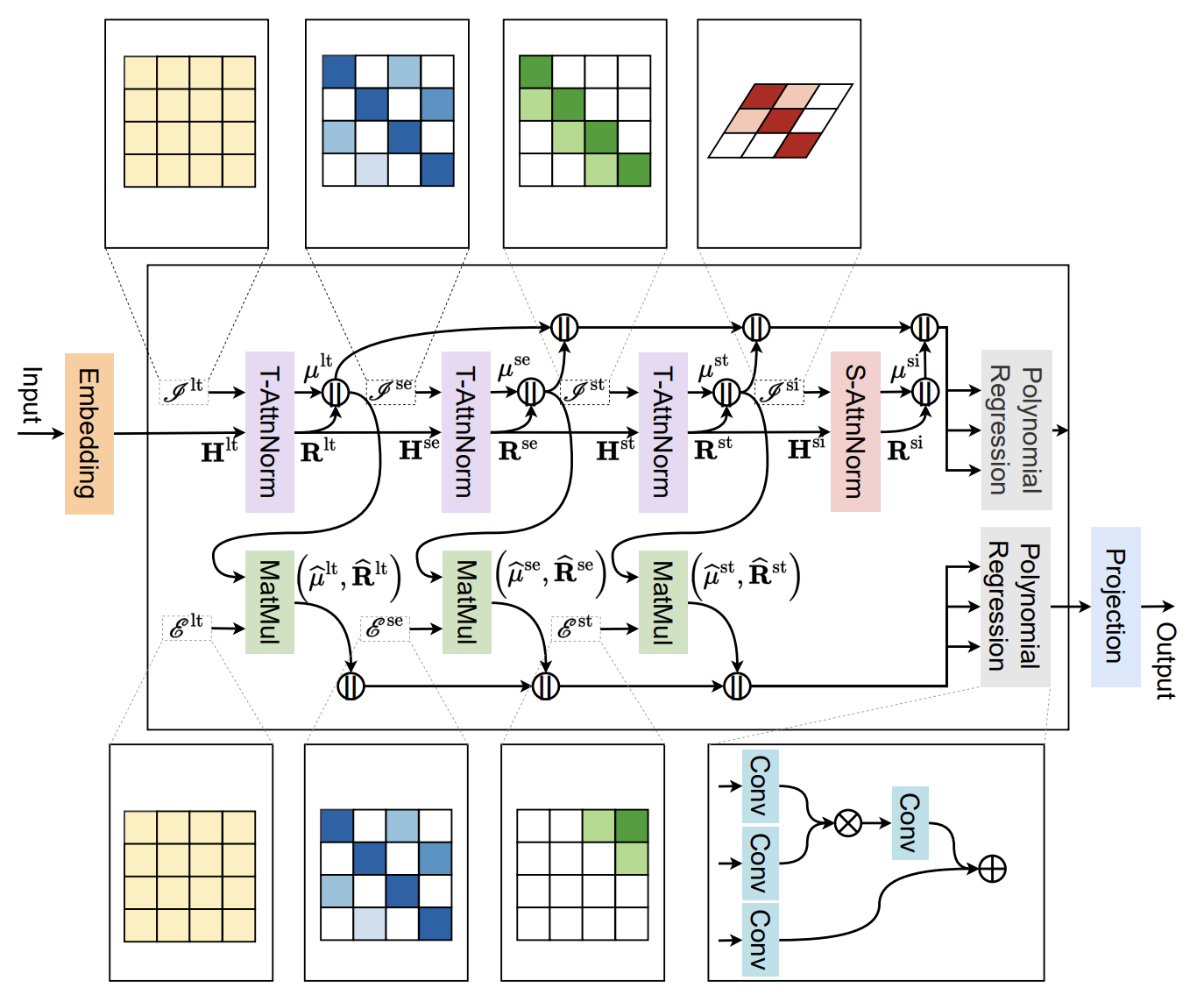
The SSCNN architecture is organized into two functionally distinct branches. The upper branch is responsible for the inference process: it extracts the structural components of the time series along with the corresponding residuals. The lower branch, in turn, focuses on extrapolation — that is, on predicting how these components might evolve over time.
The resulting components and residuals are combined into a single wide vector, which is then fed to the polynomial regression layer. This layer makes it possible to identify complex relationships between elements while preserving the structural labeling of the data.
The authors of the SSCNN framework introduce a new normalization mechanism, T-AttnNorm, based on temporal attention. It makes it possible to identify the main components of a time series step by step: the long-term, seasonal, and short-term components. Each of these elements is extracted individually for each variable along the time axis. At the same time, an attention map (selection map) is formed, reflecting the dynamics of the component of interest.
After extracting the component, the model separates it from the overall representation of the series, yielding a residual signal that contains the information not included in the structure of the extracted element. Thus, from the initial representation of the time series H ∈ RN*Tin*d, two streams are formed: the structural component µ ∈ RN*Tin*d and the residual R ∈ RN*Tin*d. The selection map I ∈ RN*Tin*Tin governs the formation of each component.


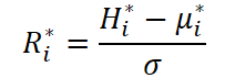
To ensure correct normalization, the rows of the matrix I* are normalized so that each row sums to 1. The difference between the long-term, seasonal, and short-term components lies precisely in the way this matrix is constructed.
It is important to note that the residual obtained at one stage is fed to the input of the next block. For example, to isolate the seasonal component, the residual remaining after the long-term component has been removed is used as the input.
Once each structural component and the residual signal have been decomposed, both streams are extrapolated to the future time horizon using a linear mapping defined by the matrix E* ∈ RN*Tin*Tout. Like the attention map I*, the matrix E* is also row-normalized.

As a result, we obtain the predicted components ̂µ* and R̂* ∈ RN*Tout*d.
The long-term component of the model is used to identify and describe sustained trends in time series. To obtain the most objective assessment of this component, the framework's authors average the values collected over several seasons. This approach minimizes the impact of seasonal and short-term fluctuations, which have only a localized effect and can distort the overall trend.
The mechanisms for isolating and extrapolating the long-term component are implemented using simple matrices whose entries are all equal: each cell of such matrices takes the value 1/Tin. This means that each time point in the past contributes equally to the long-term picture. Thus, no single segment of the series is given priority — on the contrary, the model relies on global, averaged behavior.
The framework's authors deliberately excluded the attention mechanism (attention) from the processing of the long-term component. Experience has shown that, in the datasets under consideration, this does not lead to an increase in forecast accuracy. Attention can indeed be useful when the distribution of a component changes significantly over time — in such cases, it helps reduce the bias in the estimate. However, in the case of the long-term component, this distribution remains stable throughout the entire input interval. Therefore, using attention in this context is unjustified and merely adds unnecessary complexity with no practical benefit.
The seasonal component of the model is designed to describe regular fluctuations that recur with a specified periodicity. Its extraction is based on the assumption of a stable cycle length, which simplifies the identification of seasonal patterns. Here, the notation c is introduced as the length of one cycle. Then τin denotes the number of complete cycles contained in the sequence under analysis (τin • c ≤ Tin), while τout denotes the minimum number of cycles required to cover the output sequence (τout • c ≥ Tout). For convenience in subsequent calculations, we assume that the input length Tin is a multiple of c.
To obtain an accurate and unbiased estimate of the seasonal component, the authors of the SSCNN framework introduce a trainable parameter matrix Wse ∈ Rτin*τin, where each cell reflects the relationship between a pair of cycles. This matrix is normalized row by row using SoftMax. Thus, when calculating the weights for the current cycle, the contributions of all previous cycles are taken into account, which makes it possible to capture both local and global patterns.
The model constructs a special selection map — a kind of filter — that allows it to extract only those values that correspond to identical phases in different cycles. In other words, only the first days of each month, for example, or only the Mondays of each week are compared — depending on the scale of the cycle. This is achieved by considering only elements whose index difference is a multiple of c, while membership in a particular cycle is determined using integer division.
When moving on to extrapolation — that is, when forecasting the seasonal component for future time points — similar logic is applied. A matrix Ŵse ∈ Rτout*τin is introduced, reflecting the relationships between cycles in the output and input sequences. It is also normalized and generates a selection map for extrapolation, ensuring a logical and consistent extension of the already identified seasonal patterns into the future.
This arrangement allows the model to accurately account for recurring data structures and use them as an anchor for predictions, ensuring high robustness and accuracy in seasonal forecasts.
The short-term component is designed to identify local anomalies and short-term effects that fall outside the scope of seasonal and long-term patterns. Unlike the trend, it is formed based on a limited observation window δ, which determines the depth of the temporal lookback. Such data remain relevant only in the short term and show varying degrees of correlation depending on the lags — that is, the distance between observation points.
This is precisely why the extraction of the short-term component is based on the parameter vector wst ∈ Rδ, which allows the values within a given window to be weighted differently. These weights undergo SoftMax normalization, which helps emphasize the most significant observations while preserving the numerical stability of the model. Thus, attention is focused solely on the most recent values in the time series, ensuring a focus on the changes closest to the forecast.
When it comes to forecasting the short-term component, the approach depends on how far into the future the time horizon extends. If the prediction covers the next few steps, correlations with recent values are retained, and a regression model based on the parameter matrix wst ∈ Rδ*δ is used. However, as the model moves to more distant horizons, uncertainties accumulate, reducing the reliability of forecasts. In such cases, the model uses the zero-padding method, deliberately discarding redundant parameters that could lead to overfitting.
Thus, the short-term component remains compact and flexible, accurately capturing local fluctuations without overcomplicating the model with unnecessary computations and weights. This adaptability is particularly important when dealing with unstable or noisy data, where short-term dynamics play a key role in decision-making.
The spatial component encompasses those aspects of time series that cannot be described using the previously identified time structures — long-term, seasonal, and short-term. In other words, it reflects features that are temporally irregular but spatially consistent, and that manifest themselves in a similar way across several series simultaneously.
This component is extracted using a special normalization mechanism based on spatial attention — S-AttnNorm. Unlike temporal normalization, which is applied along the time axis, here the processing is performed frame by frame, along the spatial dimension. In other words, at each time step, the model analyzes the behavior of all time series simultaneously, identifying their common characteristics.
The calculations are organized similarly to temporal normalization: for each frame, the mean (centroid), standard deviation, and residual component are calculated. Here, however, vectorization is performed orthogonally to the time axis — each time step is treated as a cross-section in space.
Correlation analysis is used to identify relationships between time series, particularly those that persist after the removal of the main temporal structures (trend, seasonality, and short-term dynamics). Each time series is represented as a Tin × d matrix, which is then vectorized. This allows us to construct a similarity matrix Isi ∈ RN×N that reflects the conditional correlation between pairs of series. Thus, the model is able to identify groups of time series that respond to external factors in a similar way, despite the temporal instability of these responses.
Upon completing the decomposition of the temporal and spatial components, the model proceeds to the aggregation and interpretation stage, where the extracted components are combined into a unified representation for the final forecast. This stage is implemented using a polynomial regression layer — a key component of the architecture that allows for both linear and nonlinear interactions between components.
In their implementation, the authors of the SSCNN framework significantly expanded the module’s functionality: additive (summing) relationships are augmented with multiplicative dependencies, making it possible to model more complex forms of relationships between components, including second-order effects.


The vector Si represents the concatenation of all previously obtained components and their corresponding residuals.
This structure allows the layer not only to sum the extracted features, but also to identify their interdependencies and combined effects, which is particularly important in the context of high-dimensional, interrelated time series.
The processing result, Hi, is a generalized representation that already takes all key patterns into account. This representation is passed to the next level of the model, starting with a new iteration of the long-term block Hlt i , thereby closing the architectural loop and ensuring coherent predictive dynamics. This approach enhances the model's expressiveness and its ability to be finely tuned to real market data, where simply adding the components often proves insufficient.
An author-created visualization of the SSCNN framework is shown below.
Implementation in MQL5
After taking an in-depth look at the theoretical foundations of the SSCNN framework, we now move on to the practical part of the article. Here, we will examine in detail one implementation of the proposed methods using the capabilities of the MQL5 environment. This will allow us to solidify these conceptual ideas and demonstrate their effective application in real-world financial market conditions.
While studying the theoretical section, you might have already noticed the striking conceptual similarity between the SSCNN framework presented here and the SCNN approach we discussed earlier. This similarity is even reflected in the names of the frameworks, which is no coincidence. Both methods are based on the idea of decomposing a time series into separate components, allowing for a more nuanced and structured analysis of the data.
However, the key difference lies in the approach itself to identifying these components and then extrapolating them. While SCNN uses more traditional decomposition and forecasting methods, SSCNN incorporates innovative adaptive mechanisms, such as selective structured decomposition and specialized attention maps, which significantly improve forecast accuracy and efficiency.
That said, extracting the long-term component using a matrix filled with identical fixed values essentially amounts to classical normalization — averaging over the entire time interval. This simplifies the task and makes it possible to use tried-and-tested, ready-made solutions without having to invent something new.
At the same time, the situation changes when it comes to identifying more complex components — the seasonal and short-term components. This will require significantly more effort and fine-tuning. To extract them correctly, adaptive mechanisms are needed that can capture the periodicity, variability, and local characteristics of the time series. This involves constructing specialized attention maps, parameterizing the relationships between periods, and accounting for local correlations.
Let's move on to the key element of the implementation — writing and analyzing the forward-pass kernel in OpenCL. It is here, at the low level of the computational architecture, that the actual data processing begins, providing the fundamental normalization and attention operations without which the model’s high accuracy and stability would be impossible.
This transition is logical and necessary. We already know how important it is to carefully and consistently isolate the long-term, seasonal, and short-term components of a time series. However, in order to implement these concepts efficiently and scalably, we need a powerful tool for parallel processing of large data sets. OpenCL is exactly such a tool, providing flexible, high-performance access to the resources of modern GPUs and CPUs.
We start by creating the AttentNorm kernel, the main working module responsible for applying attention mechanisms and normalizing the input data. Its task is to take raw time-series data, weight it using a precomputed attention matrix, compute local means and standard deviations, and then perform standardization, bringing the data into a normalized form.
The kernel parameters include pointers to the data being analyzed, attention weights, arrays for means and standard deviations, and a buffer for storing the normalized results. In addition, constants are passed: the total number of elements in each sequence and the size of the segment to be processed.
__kernel void AttentNorm(__global const float* inputs,
                         __global const float* attention,
                         __global float* means,
                         __global float* stdevs,
                         __global float* outputs,
                         const int total_inputs,
                         const int segment_size
                        )
  {
   const size_t s = get_global_id(0);
   const size_t i = get_local_id(1);
   const size_t v = get_global_id(2);
   const size_t total_segments = get_global_size(0);
   const size_t total_local = get_local_size(1);
   const size_t variables = get_global_size(2);
Next, inside the kernel, we obtain the indices of the current work-items in three dimensions. The variable s refers to the global segment index, i refers to the local index within the block, and v refers to the global index of the variable or channel. These values allow each thread to know exactly which section of data it is responsible for. The total number of segments, the local block size, and the number of variables are also determined to ensure proper distribution of the work.
A local array named Temp is declared in the device's fast memory for temporary storage of intermediate results. Next, the offset is calculated — the index in the source data array that corresponds to the current thread, variable, and segment.
   __local float Temp[LOCAL_ARRAY_SIZE];
   const int shift = v * total_inputs + s * segment_size + i;
At the beginning of the calculations, variables are initialized to store the mean, standard deviation, and a temporary value, which will be accumulated gradually. Next, a loop is started in which each local thread processes the segment elements in turn with a specified stride, ensuring parallelism and an even distribution of computations. At the same time, an out-of-bounds check is performed to prevent memory access errors.
   float mean = 0, stdev = 0;
   float val = 0;
   for(uint l = 0; l < segment_size; l += total_local)
     {
      if((l + i) >= segment_size ||
         (s * segment_size + l + i) >= total_inputs)
         break;
      float val_l = IsNaNOrInf(inputs[shift + l], 0);
      if(l == 0)
         val = val_l;
      float att = IsNaNOrInf(attention[v * segment_size + l + i], 0);
      mean += val_l * att;
      stdev += val_l * val_l * att;
     }
At each iteration of the loop, a value is retrieved from the source array, taking the offset into account; a function is applied to protect against invalid data by replacing non-numeric or infinite values with zero. For the first iteration, the current value is stored in a separate variable for later use. Similarly, the corresponding weight is retrieved from the attention-weight array, and its validity is also checked.
Next, the sum of the weighted values is accumulated to compute the mean, as is the sum of the weighted squares of the values for subsequent calculation of the variance. After the loop is complete, the local summation function performs a reduction across all local threads within the block: all partial sums are combined into a single total, ensuring accurate calculation of the statistics. To ensure proper synchronization of the threads, a barrier is used to guarantee that all threads have completed their computations before proceeding further.
   mean = LocalSum(mean, 1, Temp);
   BarrierLoc;
   stdev = LocalSum(stdev, 1, Temp);
//---
   stdev -= mean * mean;
   stdev = IsNaNOrInf(sqrt(stdev), 1);
   if(stdev <= 0)
      stdev = 1;
The next step is to calculate the variance by subtracting the square of the mean from the sum of squares, and then take the square root to obtain the standard deviation. It is important to note that if the standard deviation is zero, negative, or invalid, it is replaced with one to avoid errors during subsequent normalization.
After that, one of the local threads writes the calculated mean and standard deviation to the corresponding output arrays, ensuring that the results for each segment and variable are saved.
   if(i == 0)
     {
      int shift_ms = v * total_segments + s;
      means[shift_ms] = mean;
      stdevs[shift_ms] = stdev;
     }
Then another loop is launched, during which the data normalization itself takes place: the mean is subtracted from each input value, and the result is divided by the standard deviation, with a mandatory check to ensure the result is valid. The normalized values are stored in the output buffer, ready for further processing.
   for(uint l = 0; l < segment_size; l += total_local)
     {
      if((l + i) >= segment_size ||
         (s * segment_size + l + i) >= total_inputs)
         break;
      if(l > 0)
         val = inputs[shift + l];
      outputs[shift + l] = IsNaNOrInf((val - mean) / stdev, 0);
     }
  }
This kernel efficiently distributes the workload among threads, ensures accurate calculation of statistics while accounting for attention weights, and correctly normalizes the data, which is particularly important when working with time series in forecasting and analysis tasks. The use of local memory and synchronization ensures high performance and computational stability.
In addition, it is important to note one of the key assumptions underlying this kernel’s algorithm. Specifically, it is assumed that the size of the local work-group is equal to the size of the segment being analyzed. This is not merely a formal equality, but a fundamental condition that simplifies the computational logic and improves the efficiency of code execution on the GPU.
When this condition is satisfied, the loops designed to iteratively traverse the segment in steps equal to the size of the local work-group are effectively reduced to a single iteration. This means that each thread processes exactly one element of its segment without making repeated passes. This approach drastically reduces the complexity of internal loops, simplifies the logic, and, most importantly, minimizes the number of accesses to global memory.
Instead of repeatedly reading data from the global buffer, each segment value is stored in a local variable at the first opportunity and is then accessed from a register. And this is an entirely different level of performance: accessing a register or local memory is an order of magnitude faster than accessing global memory, especially when hundreds or thousands of parallel segments need to be processed in real time.
Thus, a properly chosen ratio between the work-group size and the segment size becomes not merely a configuration element, but an active optimization factor. It makes it possible to fully unlock the potential of hardware acceleration, reducing overhead and improving the efficiency of the entire time series processing system.
Nevertheless, despite the elegance and effectiveness of the approach described, in real-world conditions one cannot rely solely on ideal scenarios. Unfortunately, the technical capabilities of hardware do not always align with our wishes. GPU platforms differ in architecture, available memory, local work-group size limits, and even driver-specific features. All of this means that strict equality between the work-group size and the segment length is more desirable than guaranteed.
That is precisely why we still keep the loop in the code — as an element of adaptability and versatility. Although it is executed only once in the optimal case, it remains necessary for situations where the hardware does not allow a local work-group of the required size to be specified. It is a kind of safeguard: if the segment turns out to be longer than the available local work-group, the loop will neatly process it in parts, ensuring correct calculations under any circumstances.
This compromise between efficiency and flexibility makes it possible to maintain performance where possible while ensuring correct operation even on less powerful devices. In the world of computing tasks, as in life, it is always worth keeping a plan “B” close at hand, especially when working with hardware that is not inclined to compromise.
After describing the forward pass, where each element is normalized based on the mean and standard deviation of its segment, we move on to a more subtle and, at the same time, critically important part — the backward pass algorithm. Simply propagating errors is not enough here. It is important to take into account that each element of the output gradient affects all elements of the input segment, since both the mean and the variance are calculated over the entire data set at once. This imposes certain implementation-specific requirements.
To make this clearer, let's take a moment to look at the expression describing the derivative of the normalized value with respect to the input.
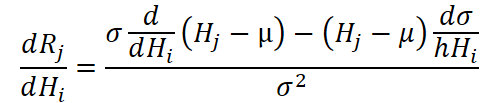
It contains two terms: one depends directly on the derivative with respect to the input value, and the other depends on the derivative with respect to the standard deviation, which in turn depends on all the values in the segment. This means that it is impossible to compute the gradient for a single element without taking into account the contributions of all the others.
Formally, this is expressed by the fact that each output gradient must be projected back onto the entire segment, not just onto its own input “cell.” Thus, to correctly compute the gradient with respect to a specific input element, it is necessary to iterate over all output elements of the segment and sum their contributions, taking into account how the mean and standard deviation would change if that input were varied.
A special case arises when the index of the current output element matches the index of the input element for which we are collecting the gradient. In that case, the effect propagates not only through changes in the statistics, but also directly — through the derivative of the normalization of the value itself. If, however, the indices differ, only an indirect effect remains, and it is entirely determined by changes in the mean values and the variance.
In the implementation, this means that for each input element, we must iterate over all the output gradients of the segment, summing the effect of each one. This approach makes the kernel structure more complex, but it achieves exact correspondence with the mathematical formulation. This is especially important if we want the neural network model to be trained correctly and efficiently.
Turning to the AttentNormGrad kernel algorithm, we find ourselves at the very heart of the backpropagation algorithm. It is here that the gradients with respect to the input data and attention weights are calculated, taking into account how the normalized output depends on the entire set of segment values.
__kernel void AttentNormGrad(__global const float* inputs,
                             __global float* inputs_gr,
                             __global const float* attention,
                             __global float* attention_gr,
                             __global const float* means,
                             __global const float* stdevs,
                             __global const float* means_gr,
                             __global const float* outputs_gr,
                             const int total_inputs,
                             const int segment_size
                            )
  {
   const size_t i = get_global_id(0);              // main
   const size_t loc = get_local_id(1);             // local to sum
   const size_t v = get_global_id(2);              // variable
   const size_t total_main = get_global_size(0);   // total
   const size_t total_loc = get_local_size(1);     // local dimension
   const size_t variables = get_global_size(2);    // total variables
At the beginning of the kernel, the indices are defined as follows:
- i — the global ID of the current element,
- loc — a local index within the work-group,
- v — the index of the variable we are working with.
   __local float Temp[LOCAL_ARRAY_SIZE];
//--- Input gradients
     {
      const int s = i / segment_size;
      const int shift_in = v * total_inputs + i;
      const int shift_ms = v * segment_size + s;
      float grad = 0;
      if(loc == 0 && i < total_inputs)
        {
         Temp[0] = IsNaNOrInf(inputs[shift_in], 0);
         Temp[1] = IsNaNOrInf(means[shift_ms], 0);
         Temp[2] = IsNaNOrInf(stdevs[shift_ms], 1);
         Temp[3] = IsNaNOrInf(means_gr[shift_ms], 0);
         Temp[4] = IsNaNOrInf(attention[(v - s) * segment_size + i], 0);
        }
      BarrierLoc;
Next comes the first part of the kernel — the calculation of gradients with respect to the input data, inputs. Here, we determine which segment the element i belongs to, calculate the necessary memory offsets, and — if we are on the first thread within the local work-group (loc == 0) — load the required values into the local buffer: the input value itself, the mean, the standard deviation, the gradient of the mean, and the corresponding attention weight. Next comes a synchronization barrier to ensure that all threads wait until the data has been loaded and can then work with it safely.
Now the most important work begins. We go through the entire segment and analyze the contribution of each normalized output to the gradient of the input value we are interested in. In this process, special attention is paid to whether the positions match— that is, whether this is the same element with respect to which we are taking the gradient (same). If so, its contribution is computed directly; if not, only indirectly, through changes in the segment statistics. To do this, the calculation takes into account both the deviation of the value from the mean and its effect on the standard deviation. All of this is carefully accumulated in the variable grad. We also take into account the gradient with respect to the mean, accumulated across other information streams.
      if(i < total_inputs)
        {
         float x = Temp[0];
         float mean = Temp[1];
         float stdev = Temp[2];
         float mean_gr = Temp[3];
         float att = Temp[4];
         for(int l = 0; l < segment_size; l += total_loc)
           {
            if((l + loc) >= segment_size ||
               (i * segment_size + loc + l) >= total_inputs)
               break;
            float out_gr = IsNaNOrInf(outputs_gr[v * total_inputs + s * segment_size + loc + l], 0);
            bool same = (i - s * segment_size) == (loc + l);
            float xl = x;
            if(!same)
               xl = IsNaNOrInf(inputs[v * total_inputs + s * segment_size + loc + l], 0);
            float dy = ((int)same - att) * (1 / stdev - (xl - mean) * att * x / pow(stdev, 3.0f));
            float dmean = (same ? IsNaNOrInf(mean_gr * att, 0) : 0);
            grad += IsNaNOrInf(dy * out_gr + dmean, 0);
           }
        }
      grad = LocalSum(grad, 1, Temp);
      if(loc == 0 && i < total_inputs)
         inputs_gr[shift_in] = grad;
      BarrierLoc;
     }
The resulting values are summed locally and written to the inputs_gr buffer.
Once we are done with the gradients with respect to the input data, we move on to the second part — calculating the gradients with respect to the attention weights. Everything here is a mirror image: the logic is the same, but the emphasis shifts. Now, for each i (segment element), we iterate over all the input data and observe how the output changes when the attention weight changes. The structure remains the same: calculating the local gradient, checking the matching conditions, and accounting for the contribution through changes in the standard deviation and the mean. And once again — a careful local sum and saving the result to attention_gr.
//--- Attention gradient
     {
      float grad = 0;
      int shift_att = v * segment_size + i;
      if(i < segment_size)
        {
         float att = IsNaNOrInf(attention[shift_att], 0);
         for(int l = 0; l < total_inputs; l += total_loc)
           {
            if((l + loc) >= total_inputs)
               break;
            int shift_out = (l + loc) + v * total_inputs;
            int s = (l + loc) / segment_size;
            int shift_in = v * total_inputs + s * segment_size + i;
            float x = IsNaNOrInf(inputs[shift_in], 0);
            float out_gr = IsNaNOrInf(outputs_gr[shift_out], 0);
            float mean = means[v * segment_size + s];
            float stdev = stdevs[v * segment_size + s];
            float mean_gr = means_gr[v * segment_size + s];
            bool same = (i - s * segment_size) == (loc + l);
            float xl = x;
            if(!same)
               xl = IsNaNOrInf(inputs[shift_out], 0);
            float dy = -x / stdev - (xl - mean) * x * x * (1 - 2 * att) / (2 * pow(stdev, 3.0f));
            float dmean = IsNaNOrInf(mean_gr * x, 0);
            grad += IsNaNOrInf(dy * out_gr + dmean, 0);
           }
        }
      grad = LocalSum(grad, 1, Temp);
      if(loc == 0 && i < segment_size)
         attention_gr[shift_att] = grad;
     }
  }
Our kernel implements the gradient expression according to the formula derived earlier. The entire code is not just a set of commands, but a finely organized system. Each thread carefully evaluates how a change in each individual input or attention weight affects the outputs of the entire group. It includes optimization through local buffers, precise synchronization, and careful handling of boundary conditions. This is exactly what a true engineering solution looks like — rigorous and well-calibrated, yet adaptable to the capabilities of the hardware and the specifics of numerical differentiation.
We have examined in detail the implementation of a key component of the SSCNN framework — the normalization module with attention — within the OpenCL program. Right before our eyes, theory was transformed into a working algorithm capable of accounting for the weight of each element and distributing that influence throughout the data structure with a precision worthy of advanced engineering. We saw how important it is to fine-tune the interaction between local and global memory, how critical it is to take into account the specifics of the hardware architecture, and why even a formally simple normalization operation becomes a full-fledged computational task in a parallel environment.
However, our journey is not yet over. Normalization is only one facet of the multi-component mechanism on which the entire SSCNN framework is based. We will continue our work in the next article. The most interesting part is just beginning.
Conclusion
In this article, we explored the theoretical aspects of the SSCNN framework, with particular emphasis on the idea of structural decomposition of a time series and the extraction of components using attention-based normalization. The framework's authors proposed a well-founded architecture capable of handling high-dimensional time series with minimal computational overhead.
In the practical section of this article, we examined in detail the implementation of one of the framework's key components — the T-AttnNorm layer. Particular attention was paid to the specifics of the forward and backward passes, as well as to interaction with global and local memory. Subtleties in the algorithm's behavior in special cases were identified, and practical comments were provided on adapting it to the OpenCL architecture.
We have laid the groundwork for implementing the full SSCNN stack and established a foundation for its trainability, confirming the importance of accurate gradient collection and derivative computation. In the next article, we will continue our journey.
References
- Parsimony or Capability? Decomposition Delivers Both in Long-term Time Series Forecasting
- Other articles in this series
Programs used in this article
| # | Name | Type | Description |
|---|---|---|---|
| 1 | Study.mq5 | Expert Advisor | Expert Advisor for offline model training |
| 2 | StudyOnline.mq5 | Expert Advisor | Expert Advisor for online model training |
| 3 | Test.mq5 | Expert Advisor | Expert Advisor for model testing |
| 4 | Trajectory.mqh | Class library | Structure for describing the system state and model architecture |
| 5 | NeuroNet.mqh | Class library | Class library for creating a neural network |
| 6 | NeuroNet.cl | Library | Code library for an OpenCL program |
Translated from Russian by MetaQuotes Ltd.
Original article: https://www.mql5.com/ru/articles/19069
Warning: All rights to these materials are reserved by MetaQuotes Ltd. Copying or reprinting of these materials in whole or in part is prohibited.
This article was written by a user of the site and reflects their personal views. MetaQuotes Ltd is not responsible for the accuracy of the information presented, nor for any consequences resulting from the use of the solutions, strategies or recommendations described.

 From Basic to Intermediate: Classes (I)
 Market Simulation: Position View (XIII)
 Market Simulation: Position View (XIV)
 From Basic to Intermediate: Queues, Lists, and Trees (V)

- Free trading apps
- Over 8,000 signals for copying
- Economic news for exploring financial markets
You agree to website policy and terms of use