Neural Networks in Trading: The Temporal Query Model (TQNet)

Introduction

Multivariate time-series forecasting in finance is a race against time, where accuracy and speed are key. Exchange rates, indices, trading volumes, interest rates, and liquidity indicators — all of these factors constantly interact with one another, forming a complex, ever-changing system. Traders, asset managers, and analysts know that to stay one step ahead, you need to understand how all the variables influence one another in real time. It is precisely this ability to see the big picture that lies at the heart of modern forecasting in financial markets.

The problem is that financial data is not like laboratory measurements taken under sterile conditions. The market has a life of its own: sharp price swings in response to news, periods of high and low volatility, and unexpected correlations that appear and disappear in a matter of hours. Add noise to the mix (measurement errors, quote delays, data gaps), and we are faced with a classic problem: how to extract a reliable signal in a world full of randomness. The situation becomes particularly complex when local relationships between parameters within a single time segment contradict the overall picture across the entire observation history. It is like trying to predict a currency's exchange rate based on just one day, when the overall trend has been moving in the opposite direction for months.

To bridge this gap, the paper "Temporal Query Network for Efficient Multivariate Time Series Forecasting" proposed a new approach called Temporal Query — a tool that makes it possible to combine local and global views of the market. It is based on trainable vectors that are cyclically shifted in time, capturing stable cross-variable relationships that have been validated by the entire history of the data. At the same time, the quotes, indicators, and other market parameters themselves serve as keys and values in a multi-head attention mechanism, accounting for the unique characteristics of each specific moment. This has a twofold effect: the model retains its ability to respond to instantaneous changes while drawing on fundamental, more stable market relationships.

Based on this principle, the Temporal Query Network (TQNet) framework was developed — a minimalist yet powerful architectural solution capable of forecasting the dynamics of a set of interconnected financial instruments. Its structure is extremely simple: just a single layer of multi-head attention and a shallow fully connected network. But behind this simplicity lies the ability to identify subtle dependencies between assets and respond to them more quickly than most traditional methods. In experiments conducted by the framework’s authors, TQNet demonstrated accuracy comparable to that of the most complex architectures, while operating at a computational speed comparable to that of lightweight linear models.

A key feature of TQNet is its ability to adapt to different forecast horizons by applying the same principle of balancing local and global dependencies. This is particularly valuable in financial markets, where situations can unfold in a matter of minutes, yet still follow long-term patterns that cannot be ignored.

In today’s financial markets, success does not go to those who see only the details, nor to those who rely solely on the big picture, but to those who know how to combine these two levels of perception. Temporal Query and TQNet offer precisely this capability and do so with an elegant simplicity worthy of a place in any serious analyst’s toolkit.

The TQNet Algorithm

At the heart of multivariate time-series forecasting (Multivariate Time Series Forecasting, MTSF) lies the goal of predicting the future behavior of several interrelated variables simultaneously. Formally, at time t, we have an observed historical sequence Xt ∈ R^C*L. Here, C represents the number of variables or channels (currency pairs, market indices, trading volumes, and other indicators), and L represents the length of the observation window (how many past data points we take into account). The task is to construct a forecast over a forecast horizon H by obtaining Yt ∈ R^C*H — a sequence of future values of the same variables.

In financial-market terms, this may involve forecasting quotes for major currency pairs over the next few hours, key index levels over the next trading days, or interest rate dynamics over a horizon of several weeks, based on historical data for the selected period. It is important to consider not only the individual temporal patterns of each variable, but also the correlations between them — after all, the market moves as a single entity, and changes in one segment can be instantly reflected in another.

To address this problem, the Temporal Query Network (TQNet) framework was proposed. Despite the simplicity of its architectural design, the framework combines two key mechanisms: the identification of inter-variable dependencies and the modeling of temporal structure.

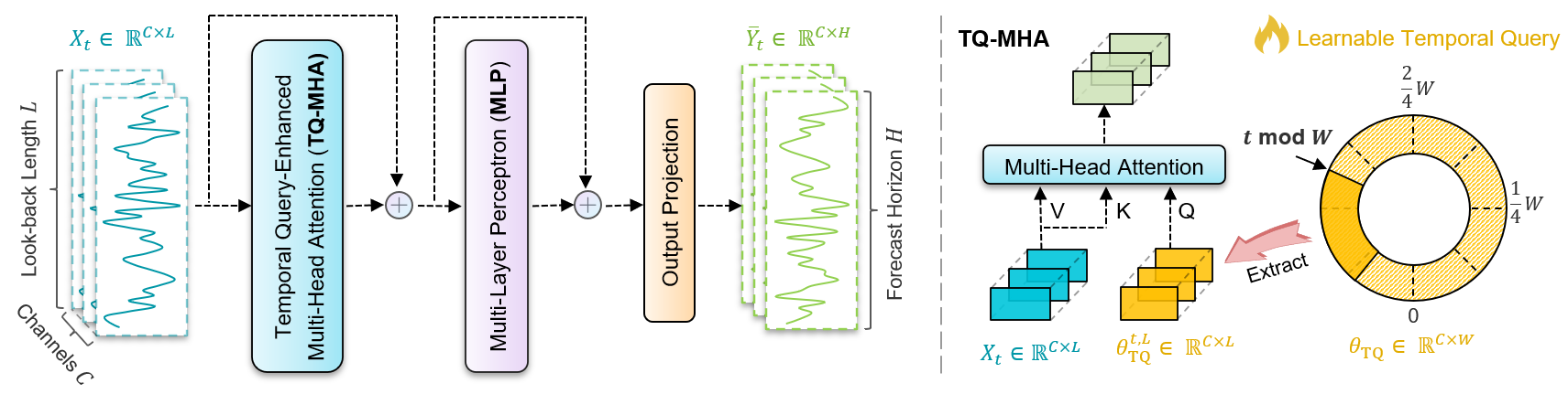
The operation of TQNet begins by feeding the analyzed sequence Xt into a multi-head attention layer enhanced by the Temporal Query (TQ-MHA) component. This layer is responsible for identifying and integrating correlations between variables — both global, globally stable correlations and local correlations specific to the current market context. The result is then processed by a shallow fully connected multilayer network (MLP), which refines the temporal dependencies and helps the model capture trends and the rhythms of change.

Both of these blocks (TQ-MHA and MLP) are equipped with residual connections, which improves training stability and reduces the risk of quality degradation on large datasets. The final stage consists of a linear layer with Dropout, which projects the obtained hidden representations onto the output space, generating a forecast Ŷt ∈ R^C*H.

A key element of the TQNet architecture is the Temporal Query (TQ) method — a specific way of forming queries (Query) within the attention mechanism. Its idea is simple and elegant: instead of deriving queries directly from the raw data, as is done in classical Self-Attention, the authors of the framework propose using a set of trainable vectors that are periodically shifted along the time axis. This approach makes it possible to capture global correlations between variables that are robust to short-term market fluctuations and noise.

Formally, given a period size W in the data being analyzed, we initialize the parameter matrix θTQ ∈ R^C×W. Here, C is the number of variables (channels), and W is the vector length that determines the periodic shift interval. These parameters are initially initialized to zeros and are adaptively adjusted during training to reflect the internal dependencies in the data. The choice of W is particularly important: in financial markets, it can correspond, for example, to the number of trading sessions in a week, recurring liquidity cycles, or other stable seasonal patterns. It can be determined either based on expert knowledge of the market or using statistical methods.

The TQ principle works as follows: for each sample being analyzed at time t, we extract a fragment of length L from the matrix θTQ, starting at the position calculated as t mod W, and, if necessary, wrap around the selection cyclically. Thus, two time points that are exactly W steps apart will have identical query vectors. This creates a periodic memory effect, allowing the model to reuse learned global dependencies and reducing the impact of random market disturbances.

In the context of finance, this can be compared to an experienced trader who remembers typical market scenarios on the same days of the week or during specific trading hours, and uses that knowledge when analyzing the current situation.

In TQNet, this approach is incorporated into the multi-head attention mechanism (TQ-MHA). Here, Queries (Query) are formed not from the source data, but from temporal TQ vectors that reflect global dependencies. At the same time, the Keys (Key) and Values (Value) are still extracted from the current sequence Xt being analyzed, preserving all the local, unique information about the market at this point in time.

The index h corresponds to the attention head number, and W h ^Q, W h ^K, and W h ^V are the trainable projection matrices.

Next, attention is computed for each head.

The results, similarly to classic Multi-Head Self-Attention, are then combined and passed through a final projection.

This combination of global Queries and local Keys/Values creates a balance between robustness to noise and adaptation to the current context. In real-world market data, where periods of calm can abruptly give way to phases of high turbulence, this balance is critical. The model does not lose its ability to respond to unique events — such as unexpected macroeconomic data or sharp market moves on news — but at the same time relies on a backbone of global dependencies that persist over time.

The goal of the proposed Temporal Query (TQ) technique is to organically integrate both global and local relationships in a time series into the attention mechanism. The idea is simple but effective: Queries (Query) are formed not directly from raw data, but from periodically shifted trainable vectors θTQ, while Keys (Key) are still extracted from the original sequence. This approach allows us to strike a balance between the overall market picture and the individual characteristics of each specific data segment.

To assess the impact of global and local dependencies in practice, the framework's authors compared three scenarios:

1. The classic approach, where Query and Key are constructed from raw data. In this case, attention captures only local, instance-specific relationships between observations.
2. The hybrid approach is the one implemented in TQNet. Here, the Query is formed from trainable TQ vectors, and the Key from the source data. As a result, both global and instance-specific dependencies are taken into account when computing attention weights, which is particularly important in financial markets, where general trends are intertwined with momentary fluctuations.
3. A purely global scheme, in which Query and Key are formed from trainable TQ vectors. This method completely ignores local variations, focusing instead on the overall structure of the time series.

Aggregated results obtained from large multivariate datasets with more than 100 variables and averaged across four forecast horizons demonstrate that the TQNet approach delivered the best performance. It combines both types of correlations. In second place is the traditional scheme with purely instance-specific relationships, while the purely global variant comes last. The takeaway is clear: the balanced integration of global and local dependencies improves forecast accuracy and model robustness, which is particularly valuable when working with dynamic financial time series.

Once the TQ-MHA layer has identified stable inter-variable relationships and integrated them with local information, a multilayer perceptron (MLP) comes into play. Its task is to further process the already extracted features in the temporal dimension, capturing trends, rhythms, and lags in the interrelationships.

Despite its simplicity, MLP remains a surprisingly effective tool for identifying temporal patterns. In the TQNet architecture, it is implemented as a lightweight version: just two fully connected layers with the GeLU activation function, which provides smoother signal processing than ReLU, especially amid complex market fluctuations.

From a financial perspective, this step can be compared to a situation where an analyst, having received a summary of key market relationships, performs an additional review: identifying intraday patterns, assessing the amplitude of fluctuations, and detecting inertia and reversal points.

The resulting representations are then passed to the output projection layer. A linear transformation is applied here to adapt the internal representations to a specific forecast horizon H. Additionally, Dropout can be used to reduce overfitting and improve the model's robustness.

TQNet places special emphasis on robustness to data distribution shifts — a phenomenon that is extremely common in the financial sector. Exchange rates, commodity prices, and stock indices — all of these can undergo sharp changes in their statistical characteristics in response to news, macroeconomic factors, or regulatory decisions. If a model is anchored to an old distribution, its forecasts quickly lose relevance.

To avoid this, the TQNet framework uses Reversible Instance Normalization (RevIN) — a method that has been proven effective in a number of modern architectures. The idea is that, before processing, the model subtracts the mean and divides the data by the standard deviation, and after generating the forecast, it returns the data to their original scale. In trading terms, this can be likened to how an experienced analyst always revises their reference points when market conditions change. Normalization removes short-term shifts in scale and volatility, allowing the model to focus on patterns rather than random fluctuations in the scale of price quotes.

Thus, in TQNet, the MLP and the result projection act as the final polish on the forecast. TQ-MHA provides the skeleton of inter-variable dependencies, the MLP refines them over time, and normalization protects against statistical skews. As a result, the model produces a forecast that simultaneously takes into account the local characteristics of the current moment and maintains global market consistency.

The authors’ visualization of the TQNet framework is shown below.

Implementation in MQL5

Now that we have covered the theoretical foundations of the TQNet framework and demonstrated why combining global and local correlations can improve forecasting accuracy, it is time to move from theory to practice. We can now focus on one way to implement these ideas in the MQL5 environment, adapting the architecture for time-series analysis and forecasting in financial markets.

Here, every element — from forming Queries and Keys to data normalization and result projection — will be implemented in code. This will allow us to demonstrate how theory is transformed into a tool ready for real-world trading. This approach will allow us to test the effectiveness of TQNet with live quotes and evaluate its robustness across different market phases: from calm sideways markets to rapid trends.

Drawing on our experience in building various attention modules, we can conduct a substantive comparison between TQNet and the classic Cross-Attention block. In the traditional cross-attention scheme, cross-attention operates on tensors of queries (Queries), keys (Keys), and values (Values), which are formed from different data sources. This approach allows one sequence to selectively process the information contained in another sequence, identifying the relationships between them.

In the case of TQNet, this principle is adapted more subtly and purposefully for time-series forecasting tasks. Here, the roles of the data sources are assigned so that Queries can carry global, generalized information encoded in the trainable vectors θTQ, while Keys maintain a connection to the local structure of the source data. This combination plays a key role in financial markets, where general patterns — such as seasonality or recurring macroeconomic cycles — must be integrated with local fluctuations — sharp price spikes, market noise, and short-term imbalances in supply and demand.

Thus, TQNet can be viewed as a kind of hybrid cross-attention mechanism, in which the model’s global memory and instantaneous market signals are integrated into a single mechanism. This not only broadens the range of interrelationships taken into account, but also makes the model more resilient to abrupt regime shifts, which is particularly valuable in conditions of high volatility in currency, stock, or commodity markets.

In this regard, we are faced with a key task: forming and training a global-correlation parameter tensor, which will be used as a data source for generating Queries. It is precisely this tensor — comprising the trainable vectors θTQ — that carries information about the global relationships between variables and serves as the foundation for correctly constructing the attention mechanism.

Training it requires a careful approach: the tensor must adapt to the data structure by capturing stable correlations, while remaining robust to noise and local outliers. For financial series, this is particularly important, since asset time series are subject to sharp fluctuations — ranging from short-term spikes in liquidity to unexpected market events.

By constructing and training such a tensor, we enable the model to utilize global market patterns when processing each new sequence. Queries generated based on this tensor act as a filter that directs the model’s attention to the most significant relationships between variables, while simultaneously integrating them with the local features of the current time segment. This enables TQNet to achieve high forecasting accuracy by combining the stability of global memory with adaptability to specific market conditions.

We already have a CParams object in our toolkit, which implements an algorithm for creating and maintaining trainable parameters. Theoretically, we could use it to construct a global correlation tensor. However, this raises the question of the efficiency of such an approach.

The fact is that multivariate time-series forecasting in financial markets requires a fairly large tensor capable of accommodating correlations over the entire cycle of the data being analyzed. On the other hand, an excessively large tensor will result in significant computational costs, which will negatively impact the training speed and the model's real-time operation.

Moreover, most of these computing resources will be used needlessly. At each step of training or forecasting, we use only a small portion of the tensor corresponding to the current time window. The remaining part stays idle, and operations on it are effectively no-ops.

At the same time, the tensor size and the number of no-op operations increase in proportion to the cycle length and the number of variables being analyzed. For financial data, where the number of channels can reach the hundreds and historical periods include thousands of time steps, this inefficiency quickly becomes a bottleneck, slowing down training and reducing the model’s overall performance.

It is therefore crucial to look for solutions that reduce unnecessary computations while keeping the model capable of capturing global correlations without any loss of accuracy.

In search of a more efficient solution, we decided to somewhat rethink our approach to storing and updating correlation parameters. Instead of using a single static CParams object to generate the entire tensor, we created a modified version of that object and implemented an array of internal trainable parameter objects in it.

Each element of the array now corresponds to a separate time step, allowing us to use only the data and parameters that are relevant to the current forecast window. This approach significantly reduces unnecessary computations while preserving the model's ability to capture global relationships between variables throughout the entire analysis period.

In other words, we have obtained a dynamic parameter tensor in which each element corresponds to a specific point in time, and unnecessary operations on the other steps are completely eliminated. This makes our TQNet implementation much more resource-efficient and scalable for large financial datasets.

Now that we have examined the concept of a dynamic parameter tensor and justified the need to use an array of objects for each time step, the next logical step is to consider a specific implementation of this approach in code. The CCircleParams class plays a key role in our architecture; it inherits its base functionality from the fully connected neural layer CNeuronBaseOCL.

class CCircleParams  :  public CNeuronBaseOCL
  {
protected:
   CLayer            cOnes;
   CNeuronBaseOCL    *cCurrent;
   //---
   virtual bool      feedForward(CNeuronBaseOCL *NeuronOCL) override          { return FeedForward(); }

   ///\ingroup neuron_base_opt
   virtual bool      updateInputWeights(CNeuronBaseOCL *NeuronOCL) override   { return UpdateInputWeights(); }
   virtual bool      calcInputGradients(CNeuronBaseOCL *NeuronOCL) override   { return true; }

public:
                     CCircleParams(void) : cCurrent(NULL) {};
                    ~CCircleParams(void)  {};
   //---
   virtual bool      Init(uint numOutputs, uint myIndex, COpenCLMy *open_cl,
                          uint numNeurons, uint period, 
                          ENUM_OPTIMIZATION optimization_type, uint batch);
   virtual bool      Identity(const int rows, const int cols);
   virtual bool      Zeros(void);
   //---
   virtual bool      FeedForward(void);
   virtual bool      UpdateInputWeights(void);
   virtual bool      SetPosition(int position);
   //---
   virtual bool      Save(const int file_handle) override;
   virtual bool      Load(const int file_handle) override;
   //---
   virtual int       Type(void) override const  {  return defCircleParams; }
   virtual void      SetOpenCL(COpenCLMy *obj) override;
   virtual CBufferFloat   *getWeightsParams(void);
   virtual int       GetPeriod(void) const { return cOnes.Total(); }
   //---
   virtual bool      WeightsUpdate(CNeuronBaseOCL *source, float tau) override;
  };

This class is a specialized container for storing and managing trainable correlation parameters, ensuring that they are updated correctly and interact efficiently with the OpenCL context mechanisms, which is particularly important when working with large financial datasets on the GPU.

Within the CCircleParams class, the cOnes object plays a special role; it is a dynamic array of trainable tensors that supports the periodic nature of the object. The cCurrent parameter acts as a pointer to the active object in the array and serves as a pointer to the currently active time-step object. This allows the model to dynamically switch between contexts, processing each time segment with maximum accuracy while preserving the global dependencies accumulated over the entire analysis period.

The structure of the CCircleParams object is created and configured in the Init initialization method, which is responsible for preparing all the necessary components for the correlation-parameter tensor to function correctly.

bool CCircleParams::Init(uint numOutputs, uint myIndex, COpenCLMy *open_cl,
                         uint numNeurons, uint period,
                         ENUM_OPTIMIZATION optimization_type, uint batch)
  {
   if(!CNeuronBaseOCL::Init(numOutputs, myIndex, open_cl, numNeurons, optimization_type, batch))
      return false;

When the method is called, the inherited interfaces are first initialized by the parent class CNeuronBaseOCL, which sets the object's fundamental parameters. If an error occurs at this stage, the method immediately returns false, preventing further incorrect behavior.

Next, we prepare the dynamic array cOnes: we clear it and bind it to the OpenCL context so that all subsequent operations on tensors can be performed efficiently on the GPU.

   cOnes.Clear();
   cOnes.SetOpenCL(OpenCL);
   for(uint i = 0; i < period; i++)
     {
      cCurrent = new CNeuronBaseOCL();
      if(!cCurrent)
         return false;
      if(!cCurrent.Init(Neurons(), i, OpenCL, 1, optimization, iBatch) ||
         !cOnes.Add(cCurrent))
        {
         delete cCurrent;
         return false;
        }
      cCurrent.SetActivationFunction(None);
     }

The main loop of the method is responsible for creating an array of objects, each of which corresponds to a separate time step. For each step, a new instance of CNeuronBaseOCL is created and initialized with identical parameters specific to that step. After successful initialization, the object is added to the cOnes container, which manages all time steps. If any error occurs, the object being created is immediately deleted, which prevents memory leaks and preserves the integrity of the structure.

For each newly created neuron, the activation function is also disabled, which is important for the correlation tensor to function correctly, since the Feed-Forward stage only requires values to be passed through without any nonlinear transformation.

Once all the time-step objects have been created, the SetPosition method sets the first element of our array as the active one, establishing the initial state for further calculations.

//---
   if(!SetPosition(0))
      return false;
//---
   return true;
  }

Thus, the Init method does not simply create an array of objects; rather, it forms a structured, manageable parameter storage in which each element represents a specific point in time. This allows the model to effectively utilize global correlations, avoid unnecessary computations, and ensure readiness for training and multivariate financial time-series forecasting.

The SetPosition method plays a key role in managing the dynamic parameter tensor for correlations in CCircleParams. Its purpose is to switch the active object to a specific time step, ensuring that the model operates on the relevant data for that exact moment.

When the method is called, the cCurrent pointer is set to the element of the cOnes array corresponding to the specified position. If the selected object is missing or has not been initialized, the method returns false, signaling a problem and preventing incorrect calculations. Otherwise, when an object is successfully selected, the method returns true, confirming that the model is ready for further data processing.

bool CCircleParams::SetPosition(int position)
  {
   cCurrent = cOnes[position];
   if(!cCurrent)
      return false;
//---
   return true;
  }

Its simplicity conceals an important function: it is through SetPosition that the TQNet model can dynamically work with different time steps, activating the corresponding correlation parameters without needing to recreate or reload the entire tensor. This is particularly important for financial time series, since each new time segment requires consideration of both local and global dependencies, and effective management of the active position allows the model to remain fast and adaptive even when dealing with large amounts of data.

It should be emphasized that, during standard initialization as part of the Init method, all global correlation tensors are filled with random values. For most scenarios, this approach is perfectly acceptable: random initialization provides a variety of initial conditions and allows the trainable parameters to gradually adapt to the data structure.

However, the authors of the TQNet framework recommend a different approach — initializing the tensor with zero values. This method is particularly justified when working with financial time series, where it is important to begin training without any prior assumptions about correlations between variables, so that the model can gradually identify stable relationships based solely on historical data.

To implement this approach, CCircleParams defines the Zeros method, which sequentially sets the parameters of all time steps to zero. When this method is called, each element of the cOnes array is processed, and all values of the global correlation tensor are set to zero. This allows us to start with a clean slate for training, ensuring that the model’s initial predictions are not biased by random initial values and that the entire adaptation process is strictly determined by the data being analyzed and the structure of TQNet.

bool CCircleParams::Zeros(void)
  {
   matrix<float> zeros = matrix<float>::Zeros(Neurons(), 2);
//---
   CBufferFloat *w = NULL;
   for(int i = 0; i < cOnes.Total(); i++)
     {
      if(!cOnes[i])
         return false;
      w = cOnes[i].getWeights();
      if(!w || !w.AssignArray(zeros))
         return false;
      w.BufferFree();
      if(!w.BufferCreate(OpenCL))
         return false;
     }
//---
   return FeedForward();
  }

Thus, the Zeros method provides a convenient and effective way to control the initial state of global correlations, thereby increasing the transparency and predictability of model training on financial data.

As an alternative to zero initialization, we implement a method that allows us to initialize the global correlation tensor with an identity matrix. This approach can be useful when it is necessary to specify initially independent variables, while allowing the model to gradually uncover the actual relationships between them during the training process.

The Identity method begins by verifying that the dimensions of the matrix being created match the number of neurons in the object.

bool CCircleParams::Identity(const int rows, const int cols)
  {
   if(rows * cols != Neurons())
      return false;
   matrix<float> ident = matrix<float>::Identity(rows, cols);
   if(!ident.Reshape(rows * cols, 1))
      return false;
   if(!ident.Resize(rows * cols, 2))
      return false;
   if(!ident.Col(vector<float>::Zeros(rows * cols), 1))
      return false;

Next, an identity matrix of the specified dimensions is created, which is then sequentially reshaped and adapted to the class’s internal data structures. Special attention is paid to memory preparation and reallocation using the Reshape and Resize methods, as well as to zeroing the additional bias column to ensure correct operation when assigning values.

After the matrix has been prepared, the method iterates through all the time steps in the cOnes container.

   CBufferFloat *w = NULL;
   for(int i = 0; i < cOnes.Total(); i++)
     {
      if(!cOnes[i])
         return false;
      w = cOnes[i].getWeights();
      if(!w || !w.AssignArray(ident))
         return false;
      w.BufferFree();
      if(!w.BufferCreate(OpenCL))
         return false;
     }
//---
   return FeedForward();
  }

For each step, the weights are obtained using the getWeights method, and the contents of the prepared diagonal matrix are assigned to them. After that, the buffer in the OpenCL context is released and recreated with the new values, ensuring proper interaction with the GPU during subsequent model training.

The process is completed by calling the FeedForward method, which allows for immediate verification that the values are propagated correctly through the layer. This initialization method ensures that, at the start of training, the global correlations between variables are unbiased and begin from a neutral state, while preserving a structure that allows the model to effectively accumulate and account for actual dependencies during the forecasting process.

In a financial context, this is particularly important: the identity matrix provides a clean slate for each variable, eliminating any initial biases while allowing the model to gradually uncover stable market relationships, such as correlations between assets.

Now that we have examined in detail the initialization algorithms and methods for preparing the initial correlation parameters, it makes sense to move on to describing the forward pass algorithm — one of the key stages in the operation of the CCircleParams class.

The FeedForward method prepares the global correlation parameters corresponding to the current time step, allowing the model to update its internal states.

bool CCircleParams::FeedForward(void)
  {
   if(!cCurrent)
      if(!SetPosition(0))
         return false;
//---
   return CNeuronBaseOCL::feedForward(cCurrent);
  }

First, the method checks whether an active step is set in the cCurrent pointer. If the current object is not specified, the SetPosition method is called to automatically select the first time step in the cOnes array, ensuring that the calculations start correctly.

After the active step is set, control is passed to the method of the same name in the parent class, allowing the necessary global correlation parameters to be formed.

Thus, FeedForward serves as a bridge between the prepared global correlation tensor structure and the attention mechanism of TQNet. The proposed approach ensures flexibility and accuracy in forecasting, enabling the model to respond to both local market fluctuations and long-term trends.

Now that we have examined the forward pass mechanism and confirmed how FeedForward ensures the correct propagation of data through the active time step, the next logical step is to examine the UpdateInputWeights method, which is responsible for updating the model’s parameters.

This method plays a key role in training: this is where the weights and correlation parameters are adjusted based on the computed gradients, allowing the model to gradually adapt to the structure of the data. In CCircleParams, the method is implemented by delegating control to the identically named method of the parent class, with the active time-step element specified.

bool CCircleParams::UpdateInputWeights(void)
  {
   return CNeuronBaseOCL::updateInputWeights(cCurrent);
  }

Passing a pointer to the current time-step object ensures that the update is performed only for the relevant segment of the tensor. This improves efficiency and prevents unnecessary calculations for the remaining time steps.

It should be emphasized that, at this stage, we deliberately do not check the validity of the pointer in the cCurrent variable. This is intentional. It is extremely important that the model use the same time-step object during both the forward pass and the backward pass. Any redefinition of this object during the weight update process could disrupt the consistency of the calculations and lead to errors in parameter adaptation.

In this case, the parent class’s method is responsible for ensuring that the pointer is valid. If an error occurs, it will simply return false, preventing the weights from being updated incorrectly. This approach allows us to focus on the core process of updating the parameters of the current time step, without extra overhead or the risk of disrupting the structure of the global correlation tensor.

This is particularly important for financial time series. The model reliably operates on the current data at each step while preserving global patterns, ensuring forecast accuracy and training stability even amid dynamic and noisy market changes.

I think you have noticed that we skipped the step of backpropagating the error gradients down through the model. Instead, the calcInputGradients method is overridden with a stub implementation that always returns a successful result. This approach may seem unusual, but it is quite sufficient for updating the global correlation parameters. The model only needs to know the error gradients at the layer output level in order to adjust the weights of the current time step.

The underlying data is not involved in the calculations, since the CCircleParams object essentially does not work with external source inputs. Propagating gradients to this level makes no sense.

Using a stub implementation plays an important role here: it allows a new object to be integrated into the overall model structure while maintaining compatibility with other network components and ensuring that weights can be updated correctly without placing an unnecessary load on the system.

Taken together, these capabilities transform CCircleParams from an abstract idea of a dynamic global correlation tensor into a full-fledged, controllable object that can be effectively integrated into TQNet. The model is able to simultaneously capture stable global patterns and account for local data characteristics at each time step. This is particularly important for financial markets: the model learns to recognize recurring seasonal cycles and stable correlations between assets, as well as to respond to short-term fluctuations, market noise, and sudden events.

We've put in a lot of work, and the article has already grown to a substantial length. All of the above takes time for the information to be absorbed and to sink in. It is time to take a short break to reflect on what we have covered so far.

In the next article, we will continue our work by moving on to the development of attention algorithms and the full integration of TQNet components, demonstrating how the structures and methods described are transformed into an effective tool for forecasting financial time series.

Conclusion

In this article, we explored the TQNet framework, which combines modularity, flexibility, and high performance. This makes it a particularly valuable tool for forecasting and analyzing financial time series. The framework's architecture is designed so that each component performs a clearly defined role, and replacing or upgrading individual components does not require a complete overhaul of the entire system.

The practical portion focused on implementing the new CCircleParams object, designed to manage global-correlation parameters. We examined its initialization process and the organization of time steps in detail, and also developed alternative algorithms for setting the initial tensor values. Particular attention was paid to building the forward pass, the weight-update mechanism, and the synchronization of computations between time steps.

Thus, we have created a flexible and reliable framework component that is ready for full-scale use within more complex models. In the next article, we will focus on building a unified computational pipeline and test it on historical data to assess the system’s effectiveness and robustness under real financial market conditions.

Links

• Temporal Query Network for Efficient Multivariate Time Series Forecasting
• Other articles in this series

Programs used in the article

#	Name	Type	Description
1	Study.mq5	Expert Advisor	Expert Advisor for offline model training
2	StudyOnline.mq5	Expert Advisor	Expert Advisor for online model training
3	Test.mq5	Expert Advisor	Expert Advisor for model testing
4	Trajectory.mqh	Class library	Structure describing the system state and model architecture
5	NeuroNet.mqh	Class library	Class library for creating a neural network
6	NeuroNet.cl	Library	Code library for the OpenCL program