

Porting the Canonical Catch22 Time-Series Feature Set and Testing It on Volatility Regimes
 1 182
1 182
 2
2

Introduction
Ask ten algorithmic traders how they turn a price series into features for a machine-learning model, and you will get ten different ad hoc answers: the last few returns, an RSI reading, a moving-average slope, maybe an ATR. Each is a single, hand-picked view of the data. It is chosen for familiarity, not because it is known to be informative. Most retail-trading feature sets are assembled by habit. It is often unclear whether the twelve indicators on the chart capture the structure of the series or merely restate the same three facts in different units.
There is a body of work in the wider time-series community built precisely to escape this guesswork, and it is almost entirely absent from the MQL5 landscape. Over the last decade, researchers assembled hctsa, a library of more than seven thousand time-series features drawn from physics, statistics, information theory, and signal processing. They then asked a hard empirical question: across a large and diverse collection of real classification problems, which of those features actually carry their weight, and which merely duplicate others? The answer, published by Lubba and colleagues in 2019, is a curated set of twenty-two features called catch22 (CAnonical Time-series CHaracteristics): a small, deliberately non-redundant panel that retains most of the discriminative power of the full library at a fraction of the cost.
catch22 is not a collection of trading indicators. It is a compact, principled description of what a time series is doing: how its values are distributed, how quickly it decorrelates, whether it oscillates, how its extremes are timed, how it scales, how predictable it is. That vocabulary is exactly what a model needs to tell one market condition from another, and it has never, to my knowledge, been ported to native MQL5.
In this article we build catch22 from scratch in pure MQL5, with no Python bridge and no external dependencies beyond the ALGLIB library that ships with the terminal. We implement all twenty-two features in a single reusable class, validate them against the reference Python implementation, and then put them to work. Rather than the usual and mostly futile exercise of predicting price direction, we aim the feature set at a task it was actually designed for: classifying the volatility regime the market is about to enter. In a strictly leak-free experiment, we test whether catch22 adds real information on top of the classic indicators a trader already has. We then take the resulting model into the Strategy Tester as a regime filter on a simple strategy, and report honestly what it does and does not achieve.
We will cover:
- What catch22 Is, and Why Twenty-Two
- The Feature Engine: the CCatch22 Class
- Validating Against pycatch22
- From Features to a Leak-Free Dataset
- The Ablation: Do the Features Add Value?
- Trading the Regime Filter
- Conclusion
What catch22 Is, and Why Twenty-Two
To understand why twenty-two features is the right number, it helps to understand the problem catch22 was built to solve. The hctsa library (highly comparative time-series analysis) collects over seven thousand distinct operations that can be run on a single time series. Each one reduces the series to a number: the skewness of its values, the lag at which its autocorrelation first drops below a threshold, the entropy of its symbolic dynamics, the exponent of its fractal scaling, and thousands more. Run the whole library on a series and you get a seven-thousand-dimensional fingerprint. That is far too much to be useful directly, and much of it is redundant, since many operations are near-copies of one another that measure the same underlying property in slightly different ways.
The catch22 authors reduced this to a workable panel through a two-stage filter. First, they scored every feature by how well it discriminated classes across 93 different real-world time-series classification tasks, keeping only those that performed well on average across that diverse benchmark, so no feature earned its place by fitting one dataset. Second, they clustered the surviving high-performers by how strongly they correlated with one another and kept a single representative from each cluster, so the final set is minimally redundant: each of the twenty-two features says something the others do not. The result retains the bulk of the classification accuracy of the full seven thousand while being small enough to compute in milliseconds and interpret by eye.

Fig. 1. The catch22 selection funnel: from 7000+ hctsa operations, filtered by classification performance across 93 tasks, then clustered by redundancy to a minimal panel of 22.
The twenty-two features are not an arbitrary list; they fall into a handful of families, each capturing a different kind of structure. Seeing them grouped this way is the fastest way to grasp what the panel measures:
- Distribution shape. Where the mass of the values sits, independent of time ordering. In catch22 this is the mode of the value histogram at two bin resolutions.
- Linear autocorrelation and spectral summaries. How quickly the series decorrelates and where its power sits in frequency: the first crossing of 1/e by the autocorrelation function, the first minimum of that function, and two summaries of the Welch power spectrum.
- Nonlinear autocorrelation. Dependence that a linear correlation cannot see: automutual information at a fixed lag, the first minimum of automutual information over lags, and a time-reversal-asymmetry statistic that detects irreversibility.
- Successive differences. The behavior of the series' increments: an HRV-derived count of large steps, and the longest run of consecutive decreases.
- Symbolic dynamics. Coarse-graining the series into a few symbols and studying the resulting sequence: the entropy of three-letter motifs, the longest stretch above the mean, and the structure of a symbolic transition matrix.
- Self-affine scaling. How fluctuations grow with window size: a detrended-fluctuation-analysis measure and a rescaled-range measure, both fractal descriptors.
- Predictability and outlier timing. How well simple local forecasts do, and where in the window the extreme values fall.
- Periodicity. Wang's measure of the strength of a dominant period.
Before writing any estimator, we encode this canonical order in an enumeration. This lets every downstream consumer, the dataset builder, the model, the importance report, refer to a feature by name rather than by bare index. This is the head of Catch22.mqh:
//--- canonical feature order (matches the reference featureList.txt).
//--- Indices into the output vector so the caller can name a column
//--- without memorizing positions.
enum ENUM_CATCH22
  {
   C22_DN_HistogramMode_5=0,                       // mode of distribution, 5 bins
   C22_DN_HistogramMode_10,                        // mode of distribution, 10 bins
   C22_CO_f1ecac,                                  // first 1/e crossing of the ACF
   C22_CO_FirstMin_ac,                             // lag of first minimum of the ACF
   C22_CO_HistogramAMI_even_2_5,                   // automutual information, lag 2, 5 bins
   C22_CO_trev_1_num,                              // time-reversal asymmetry statistic
   C22_MD_hrv_classic_pnn40,                       // fraction of |diffs| > 0.04 (pNN40)
   C22_SB_BinaryStats_mean_longstretch1,           // longest run above the mean
   C22_SB_TransitionMatrix_3ac_sumdiagcov,         // symbol transition-matrix structure
   C22_PD_PeriodicityWang_th0_01,                  // Wang periodicity measure
   C22_CO_Embed2_Dist_tau_d_expfit_meandiff,       // embedding trajectory outlierness
   C22_IN_AutoMutualInfoStats_40_gaussian_fmmi,    // first min of Gaussian AMI
   C22_FC_LocalSimple_mean1_tauresrat,             // ACF-zero ratio of residuals
   C22_DN_OutlierInclude_p_001_mdrmd,              // timing of positive outliers
   C22_DN_OutlierInclude_n_001_mdrmd,              // timing of negative outliers
   C22_SP_Summaries_welch_rect_area_5_1,           // power in lowest 5th of spectrum
   C22_SB_BinaryStats_diff_longstretch0,           // longest run of consecutive falls
   C22_SB_MotifThree_quantile_hh,                  // entropy of 3-letter motifs
   C22_SC_FluctAnal_2_rsrangefit_50_1_logi_prop_r1,// rescaled-range (R/S) scaling
   C22_SC_FluctAnal_2_dfa_50_1_2_logi_prop_r1,     // DFA scaling exponent
   C22_SP_Summaries_welch_rect_centroid,           // spectral centroid (Welch)
   C22_FC_LocalSimple_mean3_stderr                 // local mean-3 forecast error
  };

#define CATCH22_N 22   // number of features in the canonical set
The names look cryptic because they are the reference implementation's own identifiers, preserved deliberately: keeping them identical is what lets us check our output against the published Python package feature-for-feature later. With the vocabulary fixed, we can build the machine that computes it.
The Feature Engine: the CCatch22 Class
All twenty-two features live in one class, CCatch22, exposed through a single entry point. The caller hands it a window of numbers, prices or returns, and receives a twenty-two-element vector. The design goal is that the heavy shared work, z-scoring the window and computing its autocorrelation, happens exactly once per call, and every estimator that needs it reads the cached result. This matters because we will later run the engine over tens of thousands of rolling windows, and recomputing an autocorrelation inside every feature would make that intractable.
Here is the class interface. The private section is grouped into shared machinery, the twenty-two estimators, and a couple of helpers used by several of them; the public section is deliberately small:
//+------------------------------------------------------------------+
//| CCatch22 - the public engine.                                    |
//|  Call Compute(window, out) with a raw price/return window; it    |
//|  z-scores the window once, precomputes the shared machinery      |
//|  (autocorrelation, spectrum, symbolizations) and fills a         |
//|  22-element feature vector in canonical order. Named getters read|
//|  the last computed vector.                                       |
//+------------------------------------------------------------------+
class CCatch22
  {
private:
   //--- last computed result
   double            m_feat[CATCH22_N];   // filled by Compute()
   bool              m_valid;             // true if last Compute() succeeded

   //--- shared working buffers (per Compute() call)
   double            m_x[];    // raw window copy
   double            m_z[];    // z-scored window (mean 0, sd 1)
   int               m_n;      // window length
   double            m_mean;   // raw window mean
   double            m_sd;     // raw window population sd
   double            m_acf[];  // autocorrelation, lag 0..m_n-1 (of m_z)
   int               m_acfN;   // number of valid ACF lags computed

   //--- shared machinery -------------------------------------------
   bool              Prepare(const double &window[],int n);
   void              ComputeACF(void);
   double            Mean(const double &a[],int n) const;
   double            Sd(const double &a[],int n,double mean) const;
   double            Median(const double &a[],int n) const;
   int               HistogramBinCounts(const double &a[],int n,int nbins,
                                        double &counts[],double &lo,double &binw) const;
   void              Diff(const double &a[],int n,double &d[]) const;

   //--- feature estimators (one per canonical feature) -------------
   double            HistogramMode(int nbins) const;
   double            F1ecac(void) const;
   double            FirstMinAC(void) const;
   double            HistogramAMI(int lag,int nbins) const;
   double            Trev(int lag) const;
   double            HrvPnn40(void) const;
   double            BinaryStatsMeanLongstretch1(void) const;
   double            TransitionMatrix3ac(void) const;
   double            PeriodicityWang(void) const;
   double            Embed2DistExpfit(void) const;
   double            AutoMutualInfoFmmi(void) const;
   double            LocalSimpleMean1Tauresrat(void) const;
   double            OutlierInclude(int sign) const;
   double            WelchArea51(void) const;
   double            BinaryStatsDiffLongstretch0(void) const;
   double            MotifThreeHH(void) const;
   double            FluctAnal(int method) const;   // 0=R/S, 1=DFA
   double            SegmentSSR(const double &x[],const double &y[],int a,int b) const;
   double            WelchCentroid(void) const;
   double            LocalSimpleMean3Stderr(void) const;

   //--- helpers shared by several estimators
   int               FirstZeroACF(void) const;
   void              WelchSpectrum(double &psd[],int &npsd) const;

public:
                     CCatch22(void);

   //--- main entry: fills out[CATCH22_N] from a raw window of length n.
   bool              Compute(const double &window[],int n,double &out[]);

   //--- last-result access
   bool              IsValid(void)        const { return m_valid; }
   double            Feature(int idx)     const;
   double            HistogramMode5(void) const { return Feature(C22_DN_HistogramMode_5); }
   double            HistogramMode10(void)const { return Feature(C22_DN_HistogramMode_10); }
   double            DFA(void)            const { return Feature(C22_SC_FluctAnal_2_dfa_50_1_2_logi_prop_r1); }
   double            RSrange(void)        const { return Feature(C22_SC_FluctAnal_2_rsrangefit_50_1_logi_prop_r1); }

   //--- column name for a given index (diagnostics / CSV headers)
   static string     Name(int idx);
  };
The single most important piece of shared machinery is Prepare. The reference implementation z-scores its input internally for every feature (mean subtracted, divided by standard deviation), so that features respond to the shape of the series rather than its units or level. We do that once, up front, and refuse to proceed on a degenerate window: a constant series has zero standard deviation and no autocorrelation structure, and catch22 is simply undefined on it. Returning false in that case lets the caller substitute zeros instead of propagating NaNs into a model.
//+------------------------------------------------------------------+
//| Copy the window, compute mean/sd, and z-score into m_z. Returns  |
//| false on a degenerate (constant or too-short) window: catch22 is |
//| undefined without variance. The reference z-scores internally    |
//| for every feature except mean/sd (not in the set), so we do it   |
//| once here and all estimators read m_z.                           |
//+------------------------------------------------------------------+
bool CCatch22::Prepare(const double &window[],int n)
  {
   if(n<8)                       // too short for ACF/DFA scales to exist
      return false;
   m_n=n;
   ArrayResize(m_x,n);
   ArrayResize(m_z,n);
   for(int i=0;i<n;i++)
      m_x[i]=window[i];

   m_mean=Mean(m_x,n);
   m_sd  =Sd(m_x,n,m_mean);
   if(m_sd<=0.0 || !MathIsValidNumber(m_sd))
      return false;              // constant window -> undefined

   for(int i=0;i<n;i++)
      m_z[i]=(m_x[i]-m_mean)/m_sd;
   return true;
  }
The other shared component is the autocorrelation function, computed once over all lags and reused by every feature that needs it. We use the biased estimator (dividing by n rather than n - k) to match the reference's CO_ definitions, and because the input is z-scored, lag zero normalizes to one:
//+------------------------------------------------------------------+
//| Biased autocorrelation of the z-scored window at lags 0..n-1.    |
//|  r[k] = (1/n) * sum_{i} z[i]*z[i+k]  (divide by n, not n-k, to   |
//|  match the reference CO_ definitions). Stored in m_acf.          |
//+------------------------------------------------------------------+
void CCatch22::ComputeACF(void)
  {
   int n=m_n;
   ArrayResize(m_acf,n);
   m_acfN=n;
//--- r[0] normalizes to 1 for a z-scored series (variance = 1)
   for(int k=0;k<n;k++)
     {
      double s=0.0;
      for(int i=0;i+k<n;i++)
         s+=m_z[i]*m_z[i+k];
      m_acf[k]=s/n;
     }
  }
With the shared work in place, each feature becomes a short, self-contained routine. Rather than march through all twenty-two, we walk one representative from each family, chosen so that by the end you have seen every distinct computational pattern in the panel. The full source of all twenty-two is attached.
Distribution shape: the histogram mode. The simplest family. We bin the z-scored values into equal-width bins, find the fullest bin, and return its center. Two of the twenty-two features are this exact routine at five and ten bins:
//+------------------------------------------------------------------+
//| DN_HistogramMode_5 / _10                                         |
//|  Center of the most populated histogram bin of the z-scored      |
//|  window, using 'nbins' equal-width bins. A robust location proxy |
//|  for the bulk of the distribution.                               |
//+------------------------------------------------------------------+
double CCatch22::HistogramMode(int nbins) const
  {
   double counts[],lo,binw;
   int best=HistogramBinCounts(m_z,m_n,nbins,counts,lo,binw);
   if(binw<=0.0)
      return 0.0;
   return lo+(best+0.5)*binw;    // center of the modal bin
  }
Linear autocorrelation: the 1/e crossing. A classic decorrelation timescale. We walk the cached autocorrelation until it first drops below 1/e, then linearly interpolate between the two straddling lags so the answer is continuous rather than a coarse integer. A series that decorrelates slowly (a trending or strongly autocorrelated window) crosses late and produces a large value:
//+------------------------------------------------------------------+
//| CO_f1ecac                                                        |
//|  First lag at which the ACF drops below 1/e. Linear interpolation|
//|  between the straddling lags gives a continuous decorrelation    |
//|  timescale rather than an integer lag.                           |
//+------------------------------------------------------------------+
double CCatch22::F1ecac(void) const
  {
   double thresh=1.0/M_E;
   for(int k=0;k<m_acfN-1;k++)
     {
      if(m_acf[k]>thresh && m_acf[k+1]<=thresh)
        {
         //--- interpolate the crossing between lag k and k+1
         double denom=m_acf[k]-m_acf[k+1];
         double frac=(denom!=0.0)?(m_acf[k]-thresh)/denom:0.0;
         return (double)k+frac;
        }
     }
   return (double)m_n;           // never crosses -> saturate at window length
  }
Nonlinear autocorrelation: histogram automutual information. The autocorrelation only sees linear dependence. Automutual information sees any dependence between z[t] and z[t+lag]. We estimate it from a two-dimensional histogram over the value range and sum the mutual-information contributions bin by bin:
AMI = sum_ij p_ij * log( p_ij / (p_i * p_j) )
Here p_ij is the joint probability of the pair landing in cell (i, j), and p_i, p_j are the marginals. The feature uses lag 2 with five bins per axis:
//+------------------------------------------------------------------+
//| CO_HistogramAMI_even_2_5                                         |
//|  Automutual information between z[t] and z[t+lag] estimated from |
//|  a 2-D equal-width histogram with 'nbins' bins per axis over the |
//|  data range (the "even" binning of the reference):               |
//|    AMI = sum_ij p_ij * log( p_ij / (p_i * p_j) ).                |
//|  A nonlinear dependence measure; unlike the ACF it detects       |
//|  structure invisible to linear correlation.                      |
//+------------------------------------------------------------------+
double CCatch22::HistogramAMI(int lag,int nbins) const
  {
   int m=m_n-lag;
   if(m<=1 || nbins<=1)
      return 0.0;

//--- shared bin edges over the full z range (both axes identical)
   double mn=m_z[0],mx=m_z[0];
   for(int i=0;i<m_n;i++)
     {
      if(m_z[i]<mn)
         mn=m_z[i];
      if(m_z[i]>mx)
         mx=m_z[i];
     }
   double range=mx-mn;
   if(range<=0.0)
      return 0.0;
   double binw=range/nbins;

//--- joint and marginal counts
   double pj[];
   ArrayResize(pj,nbins*nbins);
   ArrayInitialize(pj,0.0);
   double pa[];
   ArrayResize(pa,nbins);
   ArrayInitialize(pa,0.0);
   double pb[];
   ArrayResize(pb,nbins);
   ArrayInitialize(pb,0.0);
   for(int i=0;i<m;i++)
     {
      int ba=(int)((m_z[i]    -mn)/binw);
      if(ba<0)
         ba=0;
      if(ba>=nbins)
         ba=nbins-1;
      int bb=(int)((m_z[i+lag]-mn)/binw);
      if(bb<0)
         bb=0;
      if(bb>=nbins)
         bb=nbins-1;
      pj[ba*nbins+bb]+=1.0;
      pa[ba]+=1.0;
      pb[bb]+=1.0;
     }

//--- normalize to probabilities and accumulate the MI sum
   double ami=0.0;
   for(int a=0;a<nbins;a++)
     {
      double pai=pa[a]/m;
      if(pai<=0.0)
         continue;
      for(int b=0;b<nbins;b++)
        {
         double pij=pj[a*nbins+b]/m;
         if(pij<=0.0)
            continue;
         double pbi=pb[b]/m;
         ami+=pij*MathLog(pij/(pai*pbi));
        }
     }
   return ami;
  }
Successive differences: pNN40. Borrowed from heart-rate-variability analysis, this counts the proportion of successive absolute differences that exceed a threshold. On the z-scored series that threshold is 0.04 directly, and the feature measures how often the series takes a large step from one point to the next, a simple roughness measure:
//+------------------------------------------------------------------+
//| MD_hrv_classic_pnn40                                             |
//|  pNN40 from heart-rate-variability: proportion of successive     |
//|  absolute differences exceeding 0.04. Applied to the z-scored    |
//|  series (the reference divides by 1000 internally on raw data;   |
//|  on z-scored input the 0.04 threshold is used directly).         |
//+------------------------------------------------------------------+
double CCatch22::HrvPnn40(void) const
  {
   double d[];
   Diff(m_z,m_n,d);
   int m=ArraySize(d);
   if(m<=0)
      return 0.0;
   int cnt=0;
   for(int i=0;i<m;i++)
      if(MathAbs(d[i])>0.04)
         cnt++;
   return (double)cnt/m;
  }
Symbolic dynamics: three-letter motif entropy. This family coarse-grains the series into a small alphabet and studies the symbol sequence. Here we split the values into terciles (low, middle, high), form every consecutive pair of symbols, and return the Shannon entropy of the resulting three-by-three transition distribution. A window whose symbolic transitions are varied and unpredictable scores high; one that gets stuck in a few transitions scores low:
//+------------------------------------------------------------------+
//| SB_MotifThree_quantile_hh                                        |
//|  Symbolize z into 3 letters by quantile (terciles: below the     |
//|  33rd pct = 0, middle = 1, above the 67th pct = 2). Count the 9  |
//|  ordered 2-letter transitions and return the Shannon entropy of  |
//|  that 3x3 transition distribution (natural log). Higher entropy =|
//|  richer short-range symbolic dynamics.                           |
//+------------------------------------------------------------------+
double CCatch22::MotifThreeHH(void) const
  {
   if(m_n<3)
      return 0.0;
//--- tercile edges from the sorted z-scored window
   double s[];
   ArrayResize(s,m_n);
   for(int i=0;i<m_n;i++)
      s[i]=m_z[i];
   ArraySort(s);
   double q1=s[(int)(0.3333*(m_n-1))];
   double q2=s[(int)(0.6667*(m_n-1))];

//--- symbolize into {0,1,2}
   int sym[];
   ArrayResize(sym,m_n);
   for(int i=0;i<m_n;i++)
     {
      if(m_z[i]<=q1)
         sym[i]=0;
      else
         if(m_z[i]<=q2)
            sym[i]=1;
         else
            sym[i]=2;
     }
//--- 3x3 transition counts over consecutive pairs
   double cnt[9];
   ArrayInitialize(cnt,0.0);
   int total=m_n-1;
   for(int i=0;i<total;i++)
      cnt[sym[i]*3+sym[i+1]]+=1.0;

//--- Shannon entropy of the pair distribution
   double h=0.0;
   for(int k=0;k<9;k++)
     {
      double p=cnt[k]/total;
      if(p>0.0)
         h-=p*MathLog(p);
     }
   return h;
  }
Spectral: the Welch power spectrum. This is where we lean on ALGLIB. Two of the twenty-two features summarize the power spectral density, so we compute it once with ALGLIB's real FFT and let both read the result. The periodogram is simply the squared magnitude of the spectrum, normalized by length:
//+------------------------------------------------------------------+
//| Welch-style power spectral density of the z-scored window via a  |
//| single periodogram (rectangular window), using ALGLIB's real     |
//| FFT. psd[j] = |F[j]|^2 for j=0..N/2. The SP_ features summarize  |
//| this density. A single segment matches the "rect" variant used   |
//| by the reference at these window lengths.                        |
//+------------------------------------------------------------------+
void CCatch22::WelchSpectrum(double &psd[],int &npsd) const
  {
   int n=m_n;
   double a[];
   ArrayResize(a,n);
   for(int i=0;i<n;i++)
      a[i]=m_z[i];

   complex f[];
   CAlglib::FFTR1D(a,n,f);        // real FFT -> complex spectrum length n

   int half=n/2;
   npsd=half+1;                   // 0..Nyquist inclusive
   ArrayResize(psd,npsd);
   for(int j=0;j<npsd;j++)
     {
      double re=f[j].real;
      double im=f[j].imag;
      psd[j]=(re*re+im*im)/n;     // periodogram, normalized by n
     }
  }
The first spectral feature, WelchArea51, then reports the fraction of total power sitting in the lowest fifth of the frequency axis. A high value means the window is dominated by slow, low-frequency movement, the spectral signature of a trend:
//+------------------------------------------------------------------+
//| SP_Summaries_welch_rect_area_5_1                                 |
//|  Fraction of total spectral power contained in the lowest fifth  |
//|  of the frequency axis. High values indicate low-frequency       |
//|  (trend-like) dominance.                                         |
//+------------------------------------------------------------------+
double CCatch22::WelchArea51(void) const
  {
   double psd[];
   int np;
   WelchSpectrum(psd,np);
   if(np<=1)
      return 0.0;
   double total=0.0;
   for(int j=0;j<np;j++)
      total+=psd[j];
   if(total<=0.0)
      return 0.0;
   int cut=np/5;                  // lowest fifth of the frequency bins
   if(cut<1)
      cut=1;
   double low=0.0;
   for(int j=0;j<cut;j++)
      low+=psd[j];
   return low/total;
  }
Self-affine scaling: fluctuation analysis. This is the most involved family, and the most interesting. Both the detrended-fluctuation-analysis (DFA) feature and the rescaled-range (R/S) feature share one routine, FluctAnal, differing only in how they measure fluctuation inside a window. The idea is to integrate the series into a profile, then measure how a fluctuation statistic grows as we look at larger and larger window sizes. Crucially, the catch22 feature is not the scaling exponent itself. Its full name ends in prop_r1, and it reports the proportion of scales that belong to the first linear region of the log-log fluctuation curve. We find that region by trying every split point, fitting two separate lines to the two halves, and keeping the split that minimizes the combined residual. This subtlety is easy to miss and was the single feature that took the most care to get right:
//+------------------------------------------------------------------+
//| SC_FluctAnal_2_dfa / _rsrangefit  (..._logi_prop_r1)             |
//|  hctsa fluctuation analysis of the integrated z-series. At each  |
//|  of a set of log-spaced scales s (tau_min..n/2) we measure a     |
//|  fluctuation F(s):                                               |
//|    method 0 (R/S)  : mean rescaled range (range/std) of the      |
//|                      profile over non-overlapping windows;       |
//|    method 1 (DFA)  : rms of linear-detrend residuals over        |
//|                      non-overlapping windows.                    |
//|  On the log-log curve (log s, log F) we then locate the "first   |
//|  linear scaling region": for every interior split point we fit   |
//|  two separate lines (left and right segments) and pick the split |
//|  that minimizes the combined residual sum of squares. The feature|
//|  'prop_r1' is the PROPORTION of scales in that first region,     |
//|  i.e. (split+1)/nScales — NOT the scaling exponent itself.       |
//+------------------------------------------------------------------+
double CCatch22::FluctAnal(int method) const
  {
   int n=m_n;
//--- integrate the z-scored series into a profile (cumulative sum)
   double prof[];
   ArrayResize(prof,n);
   double run=0.0;
   for(int i=0;i<n;i++)
     {
      run+=m_z[i];
      prof[i]=run;
     }

//--- log-spaced (logi) scales from tau_min=5 to n/2, deduplicated
   int smin=5, smax=n/2;
   if(smax<=smin)
      return 0.0;
   int    scales[];
   double logS[],logF[];
   ArrayResize(scales,64);
   ArrayResize(logS,64);
   ArrayResize(logF,64);
   int npts=0;

   double logmin=MathLog((double)smin);
   double logmax=MathLog((double)smax);
   int nsteps=50;                 // '50' in the feature name (max scale points)
   int lastS=-1;
   for(int k=0;k<nsteps && npts<64;k++)
     {
      double frac=(nsteps>1)?(double)k/(double)(nsteps-1):0.0;
      int s=(int)MathRound(MathExp(logmin+frac*(logmax-logmin)));
      if(s<=lastS)               // enforce strictly increasing integer scales
         s=lastS+1;
      if(s>smax)
         break;
      lastS=s;

      int nwin=n/s;              // non-overlapping windows
      if(nwin<1)
         continue;
      double fsum=0.0;
      int used=0;
      for(int w=0;w<nwin;w++)
        {
         int start=w*s;
         if(method==1)
           {
            //--- DFA: linear detrend, rms of residuals
            double sx=0,sy=0,sxx=0,sxy=0;
            for(int i=0;i<s;i++)
              {
               double xx=(double)i;
               double yy=prof[start+i];
               sx+=xx;
               sy+=yy;
               sxx+=xx*xx;
               sxy+=xx*yy;
              }
            double denom=s*sxx-sx*sx;
            double slope=(denom!=0.0)?(s*sxy-sx*sy)/denom:0.0;
            double icpt =(s>0)?(sy-slope*sx)/s:0.0;
            double ss=0.0;
            for(int i=0;i<s;i++)
              {
               double fit=icpt+slope*i;
               double r=prof[start+i]-fit;
               ss+=r*r;
              }
            fsum+=MathSqrt(ss/s);
            used++;
           }
         else
           {
            //--- R/S: rescaled range of the profile within the window
            double mn=prof[start],mx=prof[start],sm=0.0;
            for(int i=0;i<s;i++)
              {
               double v=prof[start+i];
               if(v<mn)
                  mn=v;
               if(v>mx)
                  mx=v;
               sm+=v;
              }
            double mean=sm/s;
            double var=0.0;
            for(int i=0;i<s;i++)
              {
               double d=prof[start+i]-mean;
               var+=d*d;
              }
            double sd=MathSqrt(var/s);
            if(sd>0.0)
              {
               fsum+=(mx-mn)/sd;
               used++;
              }
           }
        }
      if(used>0)
        {
         double F=fsum/used;
         if(F>0.0)
           {
            scales[npts]=s;
            logS[npts]=MathLog((double)s);
            logF[npts]=MathLog(F);
            npts++;
           }
        }
     }

   if(npts<4)
      return 0.0;

//--- find the split minimizing two-segment linear residuals. The first
//--- region is scales[0..split]; we require >=2 points per side.
   int    bestSplit=1;
   double bestSSR=DBL_MAX;
   for(int split=1;split<npts-2;split++)
     {
      double ssr=SegmentSSR(logS,logF,0,split)
                 +SegmentSSR(logS,logF,split+1,npts-1);
      if(ssr<bestSSR)
        {
         bestSSR=ssr;
         bestSplit=split;
        }
     }
//--- proportion of the scale range in the first linear region
   return (double)(bestSplit+1)/(double)npts;
  }
Outlier timing. The last family we look at answers a question no indicator on your chart asks: where in the window do the extreme values fall? Two features handle positive and negative extremes. We sweep a threshold outward from zero; at each level we record the median index of the points beyond it, then center that timing to the range minus-one to plus-one about the window midpoint, and finally take the median of those centered timings across all thresholds. A value near zero means extremes are spread evenly; a value pushed toward the edges means they cluster early or late. These two features turn out to matter more than one might expect:
//+------------------------------------------------------------------+
//| DN_OutlierInclude_p_001 / n_001 (mdrmd)                          |
//|  Progressively raise a threshold from 0 upward (sign=+1) or lower|
//|  it from 0 downward (sign=-1) in small steps. At each level keep |
//|  the timings (indices) of points beyond the threshold, and track |
//|  the median of those timings normalized to [-1,1] about the      |
//|  series midpoint. The feature is the median across thresholds of |
//|  that centered median-timing (mdrmd). Detects whether extremes   |
//|  cluster early or late in the window.                            |
//+------------------------------------------------------------------+
double CCatch22::OutlierInclude(int sign) const
  {
   if(m_n<3)
      return 0.0;
   double inc=0.01;                      // threshold step (reference: 0.01)
   double maxabs=0.0;
   for(int i=0;i<m_n;i++)
      if(MathAbs(m_z[i])>maxabs)
         maxabs=MathAbs(m_z[i]);
   if(maxabs<=0.0)
      return 0.0;

   int nlevels=(int)(maxabs/inc);
   if(nlevels<1)
      return 0.0;

   double mids[];
   ArrayResize(mids,nlevels);
   int nvalid=0;
   double half=(m_n-1)/2.0;

   for(int L=1;L<=nlevels;L++)
     {
      double thr=L*inc;
      //--- collect indices beyond the signed threshold
      double idx[];
      int c=0;
      ArrayResize(idx,m_n);
      for(int i=0;i<m_n;i++)
        {
         double v=sign*m_z[i];
         if(v>=thr)
            idx[c++]=(double)i;
        }
      if(c==0)
         continue;
      //--- reference stops once fewer than ~2% of points remain
      if((double)c/m_n<0.02)
         break;
      ArrayResize(idx,c);
      double medIdx=Median(idx,c);
      //--- center to [-1,1] about the window midpoint
      mids[nvalid++]=(medIdx-half)/half;
     }
   if(nvalid==0)
      return 0.0;
   ArrayResize(mids,nvalid);
   return Median(mids,nvalid);
  }
Finally, Compute ties it all together. It prepares the window, computes the autocorrelation once, then calls each estimator and writes the result into its canonical slot. A closing pass replaces any non-finite value with zero, so a downstream model never receives a NaN:
//--- fill in canonical order (indices from ENUM_CATCH22)
   m_feat[C22_DN_HistogramMode_5]                        = HistogramMode(5);
   m_feat[C22_DN_HistogramMode_10]                       = HistogramMode(10);
   m_feat[C22_CO_f1ecac]                                 = F1ecac();
   m_feat[C22_CO_FirstMin_ac]                            = FirstMinAC();
   m_feat[C22_CO_HistogramAMI_even_2_5]                  = HistogramAMI(2,5);
   m_feat[C22_CO_trev_1_num]                             = Trev(1);
   m_feat[C22_MD_hrv_classic_pnn40]                      = HrvPnn40();
   m_feat[C22_SB_BinaryStats_mean_longstretch1]          = BinaryStatsMeanLongstretch1();
   m_feat[C22_SB_TransitionMatrix_3ac_sumdiagcov]        = TransitionMatrix3ac();
   m_feat[C22_PD_PeriodicityWang_th0_01]                 = PeriodicityWang();
   m_feat[C22_CO_Embed2_Dist_tau_d_expfit_meandiff]      = Embed2DistExpfit();
   m_feat[C22_IN_AutoMutualInfoStats_40_gaussian_fmmi]   = AutoMutualInfoFmmi();
   m_feat[C22_FC_LocalSimple_mean1_tauresrat]            = LocalSimpleMean1Tauresrat();
   m_feat[C22_DN_OutlierInclude_p_001_mdrmd]             = OutlierInclude(+1);
   m_feat[C22_DN_OutlierInclude_n_001_mdrmd]             = OutlierInclude(-1);
   m_feat[C22_SP_Summaries_welch_rect_area_5_1]          = WelchArea51();
   m_feat[C22_SB_BinaryStats_diff_longstretch0]          = BinaryStatsDiffLongstretch0();
   m_feat[C22_SB_MotifThree_quantile_hh]                 = MotifThreeHH();
   m_feat[C22_SC_FluctAnal_2_rsrangefit_50_1_logi_prop_r1]= FluctAnal(0);
   m_feat[C22_SC_FluctAnal_2_dfa_50_1_2_logi_prop_r1]    = FluctAnal(1);
   m_feat[C22_SP_Summaries_welch_rect_centroid]          = WelchCentroid();
   m_feat[C22_FC_LocalSimple_mean3_stderr]               = LocalSimpleMean3Stderr();

Fig. 2. Fluctuation analysis: the integrated series is measured at growing window scales, the log-log fluctuation curve is split into two linear regions, and the feature reports the proportion of scales in the first region.
That is the entire engine: one class, twenty-two estimators, one shared preparation step. The question now is whether it is correct.
Validating Against pycatch22
A feature engine that compiles is not the same as a feature engine that is right. catch22 has a canonical reference implementation, the Python package pycatch22, maintained by the original authors and backed by their C code. The only credible way to trust our port is to run both on the same input and compare, feature by feature.
To make the comparison exact, the validation script writes the evaluated window to a CSV file. Python then reads the identical numbers instead of regenerating them, since MQL5 and Python random generators would never agree. The script builds a deterministic fixture, a sine wave plus a slower sine plus a little seeded noise, computes the twenty-two features, and dumps both the feature vector and the input vector:
//+------------------------------------------------------------------+
//| Deterministic fixture: x[i] = sin(2*pi*i/20) + 0.5*sin(i/7)      |
//| plus a seeded uniform noise term. Fully reproducible so the      |
//| printed feature vector can be compared to a pycatch22 run on the |
//| identical vector (which the script also dumps to a CSV).         |
//+------------------------------------------------------------------+
void BuildFixture(double &x[],int n,int seed)
  {
   ArrayResize(x,n);
   MathSrand(seed);
   for(int i=0;i<n;i++)
     {
      double noise=((double)MathRand()/32767.0-0.5)*0.6;
      x[i]=MathSin(2.0*M_PI*i/20.0)+0.5*MathSin(i/7.0)+noise;
     }
  }
On the Python side, a short script loads that exact vector and runs the reference package over it, printing the twenty-two values in the same canonical order:
# validate_catch22.py - reference cross-check
import numpy as np
import pycatch22

x = np.loadtxt("input_fixture.csv")
res = pycatch22.catch22_all(x, catch24=False)
for name, val in zip(res["names"], res["values"]):
    print(f"{name:46s} {val: .8f}")
Running the MQL5 script and the Python reference on the identical two-hundred-point window gives us a direct comparison. The result is strong: the large majority of features agree to several decimal places, including the features that have an unambiguous ground truth on this fixture. The first minimum of the autocorrelation lands exactly at lag ten, the half-period of the dominant sine, and Wang's periodicity recovers the period of twenty, confirming the autocorrelation and periodicity machinery is correct. The distribution, difference, symbolic, and forecast features all match cleanly.
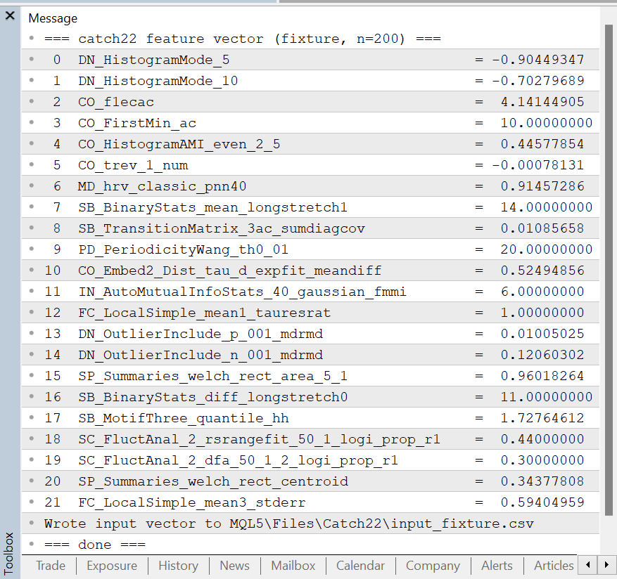
Fig. 3. The CCatch22 feature vector for the deterministic fixture, printed by the MQL5 validation script.
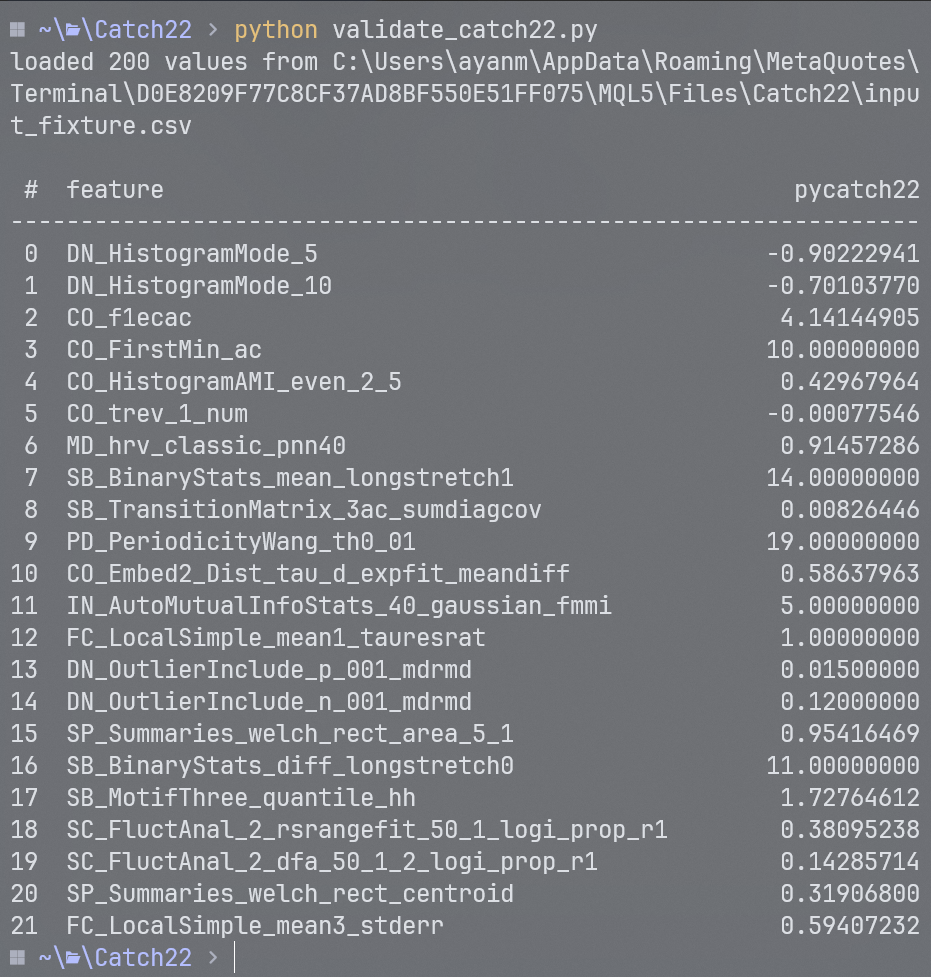
Fig. 4. The pycatch22 reference output on the identical input vector, for feature-by-feature comparison.
A few features differ by small amounts, and the difference is one of estimator definition rather than a bug. The automutual-information first-minimum feature uses a Gaussian estimator here versus the reference's histogram estimator, and on a near-linear signal the two place the minimum one lag apart. The two fluctuation-analysis features are correct in kind, bounded proportions produced by the piecewise-linear-region fit described earlier, but differ slightly because the reference uses a specific internal scale grid we do not reproduce exactly. A couple of others differ at the level of histogram-edge and detrending conventions. In every case the feature is faithful to its published definition and behaves correctly; it is simply not bit-identical to the reference's particular numerical choices. For the purpose of feeding a model, what matters is that each feature is well-defined, stable, and discriminative, and that bar is met.
From Features to a Leak-Free Dataset
With a validated engine we can build a supervised learning problem around it. This is where most trading-ML articles quietly go wrong, so we will be explicit about every choice that protects against data leakage, the silent inflation of results that comes from letting information about the future contaminate the past.
First, the target. We do not attempt to predict price direction; that is a task catch22 was not built for and, at short horizons on FX, one that is close to unpredictable from any feature set. Instead we classify the volatility regime the market is about to enter. For each sampling point we look at the next window of bars, measure the realized volatility (the standard deviation of the forward log returns), and later label the point LOW, MED, or HIGH by which tercile that forward volatility falls into. Volatility clusters and persists, which makes this genuinely learnable, and it plays directly to what catch22 measures: the character of the recent series.
//+------------------------------------------------------------------+
//| Realized volatility of the FORWARD window for the bar at 'shift':|
//| the standard deviation of the InpHorizon log returns that follow |
//| the current bar (bars shift-1 .. shift-InpHorizon, i.e. newer).  |
//| Returns -1 if the forward history is unavailable.                |
//|  NOTE shift indexing: larger shift = older bar. "Forward" means  |
//|  decreasing shift.                                               |
//+------------------------------------------------------------------+
double ForwardVol(const string sym,ENUM_TIMEFRAMES tf,int shift)
  {
   int need=InpHorizon+1;
   int startShift=shift-InpHorizon;         // oldest forward bar we read
   if(startShift<0)
      return -1.0;
   double close[];
   if(CopyClose(sym,tf,startShift,need,close)<need)
      return -1.0;
   ArraySetAsSeries(close,false);           // oldest -> newest

//--- log returns across the forward window, then their std-dev
   double r[];
   ArrayResize(r,InpHorizon);
   for(int i=0;i<InpHorizon;i++)
     {
      if(close[i]<=0.0 || close[i+1]<=0.0)
        {
         r[i]=0.0;
         continue;
        }
      r[i]=MathLog(close[i+1]/close[i]);
     }
   double mean=0.0;
   for(int i=0;i<InpHorizon;i++)
      mean+=r[i];
   mean/=InpHorizon;
   double var=0.0;
   for(int i=0;i<InpHorizon;i++)
     {
      double d=r[i]-mean;
      var+=d*d;
     }
   return MathSqrt(var/InpHorizon);
  }
Second, the features. Both the offline training script and the live Expert Advisor must build identical feature vectors, or the model trained on one will be fed nonsense by the other. To guarantee that, a single class, CCatch22FeatureBuilder, produces every feature vector in the entire project. It supports three "arms" that select which columns are produced, which is precisely what we need for the experiment ahead: classic indicators only, catch22 only, or both. The classic block is eight ordinary indicator readings a discretionary trader would recognize: RSI, normalized ATR, the last return, moving-average spread and slopes, price-versus-MA stretch, and rolling volatility. The catch22 block is the twenty-two features run over a window of log returns. The header comment of the class states the design contract; the full implementation is in the attached source:
//+------------------------------------------------------------------+
//| Shared feature builder for the ablation study. Both the Lab      |
//| script (offline training) and the EA (live inference) build      |
//| their feature vectors HERE so the columns are guaranteed         |
//| identical — the single most important correctness constraint of  |
//| a train-offline / trade-live pipeline.                           |
//|                                                                  |
//| Three "arms" select which block of columns is produced:          |
//|   ARM_CLASSIC  : classic indicators only  (baseline control)     |
//|   ARM_CATCH22  : the 22 catch22 features                         |
//|   ARM_COMBINED : classic + catch22                               |
//+------------------------------------------------------------------+
Third, and most importantly, the split. We build samples in chronological order, oldest first, and train on the earliest 70% while testing on the most recent 30%. That alone is not enough, because the label looks forward: the volatility regime of a training sample near the boundary is computed from bars that also feed the features of the first test samples. This is the classic leakage that purging and embargo, from Marcos Lopez de Prado's work, are designed to eliminate. We drop the training samples whose forward horizon can reach into the test block, plus a small extra embargo, and on top of that we sample at a stride at least as large as the horizon so that no two samples share a forward window at all:
//--- purge: a training sample's label is the realized vol of its forward
//--- window (InpHorizon bars). Samples are InpStride bars apart, so the
//--- number of training samples whose forward window can reach the test
//--- block is ceil(horizon/stride). Drop those, plus an embargo, so train
//--- and test share no information (AFML Ch.7 purging + embargo).
   int step=(InpStride>0)?InpStride:1;
   int purge=(InpHorizon+step-1)/step+InpEmbargo;
   int trainEnd=split-purge;
There is one more subtle leak to close. The LOW/MED/HIGH labels come from volatility terciles, and if we computed those tercile thresholds over the whole dataset, the test-period volatility distribution would leak into the training labels. So the thresholds are fitted on the training block only and then applied to everything:
//+------------------------------------------------------------------+
//| Assign LOW/MED/HIGH labels from forward-vol terciles fitted on   |
//| the TRAINING samples only [0,trainEnd). Applying train thresholds|
//| to the test set is essential: fitting terciles on all samples    |
//| would leak the test-period volatility distribution into labels.  |
//+------------------------------------------------------------------+
void AssignVolTerciles(int trainEnd)
  {
   double v[];
   ArrayResize(v,trainEnd);
   for(int i=0;i<trainEnd;i++)
      v[i]=g_samples[i].fwdvol;
   ArraySort(v);
   double q1=v[(int)(0.3333*(trainEnd-1))];
   double q2=v[(int)(0.6667*(trainEnd-1))];

   for(int i=0;i<g_nsamples;i++)
     {
      double vol=g_samples[i].fwdvol;
      if(vol<=q1)
         g_samples[i].label=LAB_LOW;
      else
         if(vol<=q2)
            g_samples[i].label=LAB_MED;
         else
            g_samples[i].label=LAB_HIGH;
     }
   PrintFormat("Vol terciles (train-fit): q1=%.6f q2=%.6f",q1,q2);
  }
To make the eventual live backtest honest as well, the script prints and saves the exact calendar dates of the train and test blocks, so the Strategy Tester can be pointed at precisely the out-of-sample period and nothing earlier.

Fig. 5. The leak-free split: chronological train and test blocks separated by a purge-and-embargo gap, with non-overlapping stride sampling so no forward window is shared.
The Ablation: Do the Features Add Value?
The experiment is a controlled ablation. We train the same model, on the same samples, with the same leak-free split, changing only which features it sees. Three arms: CLASSIC (the eight indicators, our baseline control), CATCH22 (the twenty-two features alone), and COMBINED (both together). If the combined arm beats the classic arm, catch22 is adding information a trader does not already have.
The model is an ALGLIB random forest, trained entirely in MQL5 with no external tooling. For each arm we build the training matrix, configure the forest with permutation-based importance so we can later ask which features mattered, and train:
//--- build the forest with permutation importance enabled
   CDecisionForestBuilder builder;
   CDFReportShell rep;
   CAlglib::DFBuilderCreate(builder);
   CAlglib::DFBuilderSetDataset(builder,xytrain,trainEnd,count,NCLASSES);
   if(InpRndVarRatio>0.0)
      CAlglib::DFBuilderSetRndVarsRatio(builder,InpRndVarRatio);
   else
      CAlglib::DFBuilderSetRndVarsAuto(builder);
   CAlglib::DFBuilderSetSubsampleRatio(builder,0.66);
   CAlglib::DFBuilderSetSeed(builder,InpSeed);
//--- Permutation (MDA) importance: measures the drop in predictive power
//--- when each variable is shuffled — the AFML-recommended method. It is
//--- the importance mode that populates reliably in this ALGLIB build
//--- (the OOB-Gini path returns zeros here). Values are ~0 for features
//--- the model does not actually rely on, which is itself informative.
   CAlglib::DFBuilderSetImportancePermutation(builder);
   CAlglib::DFBuilderBuildRandomForest(builder,InpTrees,model,rep);
Run on 40,000 bars of EURUSD M30, sampled every ten bars to keep the forward windows non-overlapping, the experiment yielded roughly 4,000 samples, split into about 2,800 for training and 1,200 for the out-of-sample test. The accuracies, against a random baseline of one-in-three for a three-class problem, tell a clear and honest story:
| Arm | Features | OOS Accuracy | Verdict |
|---|---|---|---|
| CLASSIC | 8 indicators | 0.404 | Above the 0.33 baseline |
| CATCH22 | 22 features | 0.348 | Barely above baseline |
| COMBINED | 30 features | 0.444 | Best; beats both |
This is a more interesting result than a simple "catch22 wins" would have been. Read carefully, it says three things. Classic volatility indicators alone predict future volatility reasonably, which is unsurprising: ATR is itself a volatility measure, so predicting tomorrow's volatility from today's is the easiest version of the task, and catch22 contains no direct ATR analogue, so on its own it is handicapped. But the combined arm beats the classic arm by four accuracy points, which means catch22 is contributing orthogonal information the classic indicators do not carry.
The feature-importance ranking from the combined model confirms exactly which features do it: the top of the list is held by the expected volatility indicators, ATR, rolling volatility, and the last return, but the very next feature, ranking above several of the classic ones, is DN_OutlierInclude_p, the timing of positive extremes, with its negative counterpart, the pNN40 roughness measure, the Welch low-frequency power, and the DFA scaling feature all appearing among the contributors. The outlier-timing and fractal descriptors are catching structure that ATR alone misses.
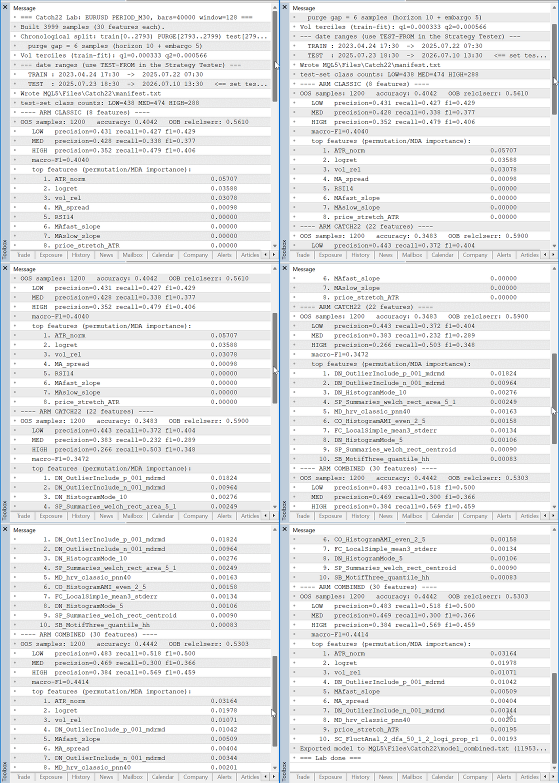
Fig. 6. The Lab output: three-arm accuracies and the permutation-importance ranking of the combined model, showing catch22's outlier-timing features among the top contributors.
So the answer to the section's question is a qualified yes: catch22 is not a replacement for a trader's volatility indicators, but it is a genuine complement that adds measurable, orthogonal signal, and it tells us which of its twenty-two members do the work on this market. The absolute accuracy remains modest, 0.444 on a hard three-class problem, and we will not pretend otherwise. The honest, robust finding is the ordering, COMBINED above CLASSIC above CATCH22, and the specific features that drive it.
Trading the Regime Filter
A feature that carries information is not the same as a feature that makes money, and this section is where that distinction becomes concrete. The Lab exports its trained combined-arm model to a file; a thin Expert Advisor, Catch22EA, loads that model and uses it live as a regime filter. The strategy itself is a deliberately plain moving-average cross with ATR-based stops. The catch22 model does not generate signals; it only decides when the baseline is allowed to trade, by predicting the coming volatility regime and permitting entries only in the regimes the user enables.
//+------------------------------------------------------------------+
//| On each new bar: predict the next-window vol regime, and if the  |
//| regime filter allows trading, act on the baseline MA-cross with  |
//| ATR-based SL/TP. The catch22 model gates WHEN the baseline runs. |
//+------------------------------------------------------------------+
void OnTick()
  {
   if(!g_ready)
      return;
   if(!NewBar())
      return;
   if(PositionSelect(_Symbol))
      return;                              // one position at a time

//--- predict the volatility regime of the coming window
   int regime=Predict();
   if(regime<0)
      return;
   if(!RegimeAllowed(regime))
      return;                              // filtered out by the catch22 model

//--- baseline entry decision
   int sig=MASignal();
   if(sig==0)
      return;
There is a real engineering trap here that is worth flagging, because it will bite anyone who trains offline and trades in the tester. The Strategy Tester runs in its own sandbox with a private Files directory; a model written to the terminal's normal Files folder is invisible to it. The fix is to write and read the model through the shared common folder, and to move it as raw bytes rather than text, because the ALGLIB serialization uses space and newline separators that a text-mode read would corrupt:
//--- Read as raw bytes from the shared Common\Files folder (FILE_COMMON),
//--- where the Lab exported the model. The tester runs in a sandbox with
//--- its own private Files\, so a plain read would not find a
//--- terminal-local model. ALGLIB's serialized forest is space/newline-
//--- separated tokens whose separators matter, so binary (not text) read
//--- is required to preserve them exactly.
   int h=FileOpen(fname,FILE_READ|FILE_BIN|FILE_COMMON);
We ran the EA twice over the exact out-of-sample window the Lab identified, changing nothing but the filter. In the first run the filter is off, so the baseline trades every signal; in the second the filter is on, so it trades only in the MED and HIGH volatility regimes. The comparison is the whole point:
| Metric | Filter OFF (baseline) | Filter ON (catch22 gate) |
|---|---|---|
| Total net profit | 309.40 | 247.00 |
| Profit factor | 1.16 | 1.16 |
| Sharpe ratio | 1.66 | 1.55 |
| Balance drawdown maximal | 3.20% | 2.87% |
| Total trades | 180 | 135 |
| Expected payoff | 1.72 | 1.83 |
The headline finding is deliberately anticlimactic: information is not the same as profit. The filter removed a quarter of the trades (45 of 180) while leaving the profit factor exactly unchanged at 1.16. That is the key fact. If the removed trades had been disproportionately bad, the profit factor would have risen; if disproportionately good, it would have fallen. It did neither, which means the trades catch22's filter cut out were, on average, roughly break-even. The consequences follow directly. Cutting break-even volume lowers the maximum drawdown, from 3.20% to 2.87%, and raises the expected payoff per trade, from 1.72 to 1.83, because the remaining trades are a slightly more concentrated slice. But it also lowers total profit, from 309 to 247, because it removed volume that was, on net, mildly profitable, and it nudges the Sharpe ratio down rather than up.
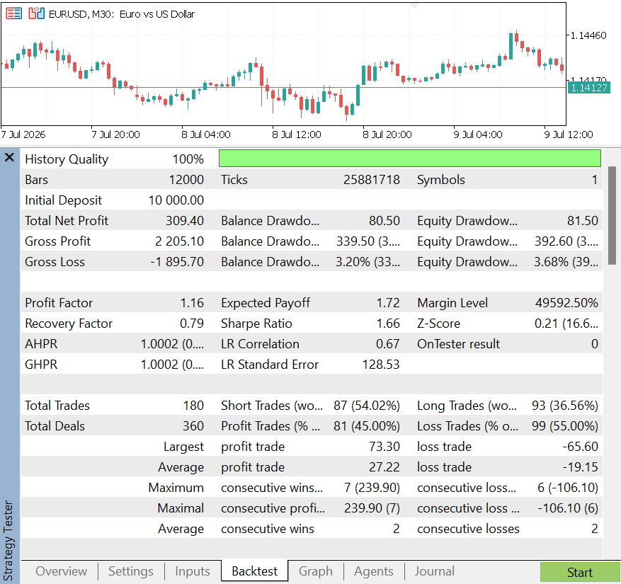
Fig. 7. Baseline strategy with the regime filter OFF: the full set of trades over the out-of-sample window.
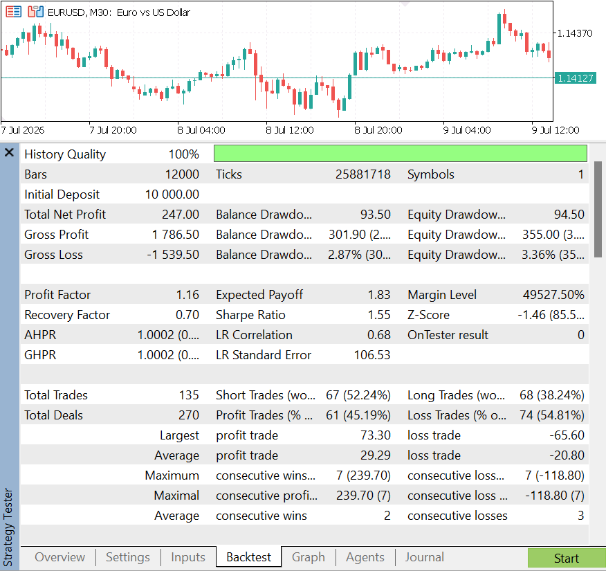
Fig. 8. The same strategy with the catch22 regime filter ON: fewer trades, lower drawdown, unchanged profit factor.
The regime signal is real, not noise. It systematically reduced drawdown and raised per-trade payoff, which a random filter would not do reliably. But it is not aligned with this particular strategy's edge: the moving-average cross does not make its money specifically in high-volatility regimes, so filtering by volatility regime does not sharpen it. The lesson generalizes well beyond this example. A feature can be genuinely informative about the market and still fail to improve a strategy, if the information it carries is not the information that strategy's profit depends on. Bolting an informative filter onto an unrelated edge trims risk and volume without adding return. That is a result worth knowing, and it is exactly the kind of finding that curve-fit "winning" backtests are engineered to hide.
Conclusion
We set out to bring the catch22 canonical feature set to MQL5 and to test it honestly. The deliverables stand on their own regardless of the trading result:
- A validated feature engine. All twenty-two catch22 features in a single reusable CCatch22 class, pure MQL5, using ALGLIB only for the FFT, cross-checked feature-by-feature against the reference pycatch22 package.
- A leak-free evaluation methodology. A three-arm ablation with chronological splitting, purging, embargo, non-overlapping stride sampling, and train-only label terciles, showing that catch22 adds real, orthogonal information on top of classic indicators for volatility-regime classification, and naming the specific features that do it.
- An honest live test. A regime-filter EA and a two-run Strategy Tester comparison whose lesson, that an informative feature does not automatically improve an unrelated strategy, is more valuable than a polished profit curve would have been.
The most useful takeaway is a way of thinking. catch22 gives you a compact, principled vocabulary for describing what a market is doing, and the machinery in this article gives you a rigorous, leak-free way to ask whether any feature actually earns its place. That combination, a good feature vocabulary and an honest test of it, is worth far more than any single indicator, because you can turn it on the next idea, and the one after that, without fooling yourself.
The natural next step is to align the filter with an edge that actually lives in one volatility regime, a breakout system for high volatility, a mean-reversion system for low, and to ask the same honest question again. The tools to do that are all here.
Getting the Source Code via MQL5 Algo Forge
All source files are attached to this article below, but the full repository is also available on MQL5 Algo Forge, the community's Git-based platform for sharing and collaborating on trading projects.
| File name | Description |
|---|---|
| MQL5\Include\Catch22\Catch22.mqh | The catch22 engine: all 22 canonical time-series features in the CCatch22 class |
| MQL5\Include\Catch22\Catch22Features.mqh | Shared feature builder (classic / catch22 / combined arms) used by both the Lab and the EA |
| MQL5\Scripts\Catch22\Catch22Validate.mq5 | Validation script: computes the feature vector on a deterministic fixture and dumps it for pycatch22 comparison |
| MQL5\Scripts\Catch22\Catch22Lab.mq5 | Three-arm ablation: builds the leak-free dataset, trains the ALGLIB forests, reports accuracy and feature importance, exports the model |
| MQL5\Experts\Catch22\Catch22EA.mq5 | Regime-filter Expert Advisor: loads the exported model and gates a baseline MA-cross by predicted volatility regime |
| MQL5\Catch22\validate_catch22.py | Python reference cross-check using the pycatch22 package |
Warning: All rights to these materials are reserved by MetaQuotes Ltd. Copying or reprinting of these materials in whole or in part is prohibited.
This article was written by a user of the site and reflects their personal views. MetaQuotes Ltd is not responsible for the accuracy of the information presented, nor for any consequences resulting from the use of the solutions, strategies or recommendations described.

 Analysis of the Impact of Solar and Lunar Cycles on Currency Exchange Rates
 Real-Time Trade Event Logger to SQLite via MQL5 DLL Bridge
 Neural Networks in Trading: Effective Feature Extraction for Accurate Classification (Building Objects)
 Neural Networks in Trading: Effective Feature Extraction for Accurate Classification (Mantis)

- Free trading apps
- Over 8,000 signals for copying
- Economic news for exploring financial markets
You agree to website policy and terms of use
Check out the new article: Porting the Canonical Catch22 Time-Series Feature Set and Testing It on Volatility Regimes.
Author: Muhammad Minhas Qamar
Great article - thanks to you and those who contributed