MQL5 Wizard Techniques you should know (Part 64): Using Patterns of DeMarker and Envelope Channels with the White-Noise Kernel

Introduction

We follow up our last article that paired momentum based DeMarker indicator with the support/resistance Envelopes bands by examining how their signals could be harnessed in machine learning. We have had similar approaches on indicator pairings in recent articles, and readers seeking some introduction can look into those. Essentially, we implement the MQL5 indicators in the Python language, while using price data imported with the MetaTrader 5 Python module. This module allows you to log onto your broker’s server and retrieve price data and symbol information.

Indicators in Python

Python has a host of technical analysis libraries that can easily be imported and use to implement a variety of indicators. The current problem is, though, that they are not all standard and some of them are missing some indicators. For instance, for this article the pandas technical analysis library is missing the DeMarker oscillator while this is available in the ‘ta’ or technical analysis module. On the other hand, the Envelopes, though present in pandas technical analysis library, is absent in the ‘ta’ library in its raw form. This is because ‘ta’ offers related indicators of Bollinger Bands and the Donchian Channel instead.

And the funny thing is, these days implementing your own indicator "from scratch" is about as much hustle (if not less) as installing one of these libraries to use these standard functions. And so, we implement our own functions for DeMarker and Envelopes, which, on paper, should allow our Python to run slightly faster given the fewer module references.

The DeMarker

The DeMarker indicator, is an oscillator that tracks the extremes of bought and sold conditions of an asset over a specified period. As already introduced in the last article it ranges between 0 and 1 with values above 0.7 implying overbought conditions, while values below 0.3 mean oversold conditions are present. We are choosing to implement it as a custom function in Python as follows:

def DeMarker(df, period=14):
    """
    Calculate DeMarker indicator for a DataFrame with OHLC prices
    
    Args:
        df: Pandas DataFrame with columns ['open', 'high', 'low', 'close']
        period: Lookback period (default 14)
        
    Returns:
        Pandas Series with DeMarker values
    """
    # Calculate DeMax and DeMin
    demax = df['high'].diff().clip(lower=0)
    demin = -df['low'].diff().clip(upper=0)
    
    # Smooth the values using SMA
    demax_sma = demax.rolling(window=period).mean()
    demin_sma = demin.rolling(window=period).mean()
    
    # Calculate DeMarker
    demarker = demax_sma / (demax_sma + demin_sma)
    return pd.DataFrame({'main': demarker})

The inputs to our function are a data-frame ‘df’ and ‘period’. The data-frame, ‘df’ is a pandas-data-frame that contains open, high, low, and close price data while period is the look back period for the DeMarker calculations. This function encapsulates the DeMarker logic while having modularity and reusability.

Calculation of DeMax provides the difference in consecutive high prices (df[‘high’].diff()). In this buffer, if the difference is positive, which would imply rising highs, it remains in the buffer otherwise the value is set to zero. This setting to zero is performed by the clip function (clip(lower=0)). Similarly, for the differences in low prices if the difference is negative(i.e., the current low is lower than the previous low), this value gets kept in the buffer as an absolute value otherwise it also sets it to zero by clipping (clip(upper=0)).

Tracking these absolute changes is important because DeMax measures upward price momentum by noting increases in high prices, while DeMin measures downward price momentum by logging decreases in low prices. These two metrics are core to DeMarker since they set by how much price moves relative to prior periods. In Python, when implementing with the diff() function it is essential to ensure input data-frame has enough data points and to be mindful that the first row will always have a NaN value.

After this, we then smooth over the values in each buffer. The smoothing reduces noise in each series and makes the indicator values less sensitive to short-term price fluctuations. The rolling(window=period).mean() method calculates the average over the specified period, and this introduces a lag that often aligns with the indicator’s purpose of identifying macro-trends. The starting period-1 values will be NaN due to insufficient data for the rolling window, and they should be handled by being dropped or filled with normalized values. The period choice also affects the DeMarker’s sensitivity, with a shorter period making it more sensitive.

We then compute the DeMarker value by dividing the DeMax mean with its value plus the DeMin mean. This step normalizes DeMarker to the 0 to 1 range, simplifying interpretation. The ratio in effect measures relative strength of upward price moves to the total price moves of both upward and downward movements. Values close to 1 indicate a strong bullish momentum, while those close to 0 imply bearish momentum is stronger.

When implementing, it is key to ensure no zero divides at this step. This is a rare occurrence though, since price is always changing, especially at the highs and lows. The function then returns DeMarker values as a pandas-data-frame with a single column that we are choosing to label ‘main’. The data-frame format ensures compatibility with other pandas based analysis tools and also allows easy integration into a larger trading system.

The Envelopes

The price-Envelopes are a support/resistance indicator that plot two bands, an upper and lower band, around a moving average of the price. The bands are offset by a fixed deviation amount in percentage, which can help traders get proxies for areas of support and areas of resistance when price touches these bands. Our Python implementation is as follows:

def Envelopes(df, period=14, deviation=0.1):
    """
    Calculate Price Envelopes for a DataFrame with OHLC prices
    
    Args:
        df: Pandas DataFrame with columns ['open', 'high', 'low', 'close']
        period: MA period (default 20)
        deviation: Percentage deviation from MA (default 0.05 for 5%)
        
    Returns:
        DataFrame with columns ['upper', 'ma', 'lower']
    """
    # Calculate moving average (typically using close prices)
    ma = df['close'].rolling(window=period).mean()
    
    # Calculate upper and lower envelopes
    upper = ma * (1 + deviation)
    lower = ma * (1 - deviation)
    
    return pd.DataFrame({'upper': upper, 'ma': ma, 'lower': lower})

Our code above provides a flexible way to compute Envelopes , with customizable periods and deviation input parameters for different strategies. The first step in calculating the Envelopes is calculating the moving average. We use a simple moving average of closing prices over the input period. The MA acts as a center line of the Envelopes and the mean price of the trend. The rolling(window=period).mean() buffer computation returns vector/buffer with mean values, but with the first period-1 values being a NaN as expected. These should be handled appropriately.

We then calculate the upper and lower band buffer values. Calculations for the upper envelope are got by multiplying the MA by (1 + deviation). For example, if our deviation is 10%, then the upper band will be 110% of the MA. Since our default deviation value is 0.1, this is equivalent to 10%. The lower envelope calculations are got by multiplying the MA by (1 - deviation) which in our case is 90%

The upper and lower bands define the price range within which price is expected to fluctuate under ‘normal’ conditions. When prices touch either band it presents scenarios of either a breakout or a reversion since we take these bands to be our support and resistance levels. These two situations pointing to trend continuations or overbought/oversold oscillations of the market.

The deviation parameter does control the width of the envelopes. A higher deviation percentage means wider bands which can be suitable for volatile assets, while a lower deviation creates a much tighter band for stable assets. This deviation should be positive to avoid invalid bands. These envelope bands are symmetrical around the MA assuming equal volatility above and below the trend. For asymmetric bands, the Bollinger can be adopted instead.

The returned pandas-data-frame features 3 columns of ‘upper’, ‘lower’, and ‘ma’. This data-frame format allows easy access to all three components, enabling visualization, signal generation or further analysis.

Features in Python

What we refer to as features are vectorized representations of the signals from the 2 indicators, DeMarker and Envelopes. These features then serve as inputs into our machine learning model, which is a recurrent neural network that uses a white noise kernel, more on that later. This machine learning implementation in python  is building on the features we first looked at in the last article that were 10 in total. Of these 10 only 6 were able to forward walk. 0,1,5,6,7 and 8. Those therefore are the features we will test through our Recurrent Neural Network (RNN). We thus have to hand code them in python before feeding them to the RNN.

Feature-0

As we saw in the last article, feature-0 aka pattern-0, generates signals based on the DeMarker crossing the overbought or oversold thresholds and price concurrently crossing the Envelopes’ upper or lower bands. We therefore implement this in Python as follows

def feature_0(dem_df, env_df, price_df):
    """
    """
    # Initialize empty array with 2 dimensions and same length as input
    feature = np.zeros((len(dem_df), 2))
    
    # Dimension 1:
    feature[:, 0] = ((dem_df['main'] <= 0.3) &
                     (price_df['close'] > env_df['lower']) &
                     (price_df['close'].shift(1) <= env_df['lower'].shift(1)) &
                     (price_df['close'].shift(2) >= env_df['lower'].shift(2))).astype(int)
    feature[:, 1] = ((dem_df['main'] >= 0.7) &
                     (price_df['close'] < env_df['upper']) &
                     (price_df['close'].shift(1) >= env_df['upper'].shift(1)) &
                     (price_df['close'].shift(2) <= env_df['upper'].shift(2))).astype(int)
    
    # Set first 2 rows to 0 (no previous values to compare)
    feature[0, :] = 0
    feature[1, :] = 0
    
    return feature

Our first line of code in the function creates a zero filled NumPy array with shape (len(dem_df), 2) that stores, categorically, bullish and bearish signals. It initializes the array, ensuring all rows default to zero. The array size must match the data-frame length to avoid index misalignment.

The bullish check index is at 0, and it gets checked first. As argued in the last article, from our implementation above, a bullish signal is generated when DeMarker is in oversold territory (typically below 0.3); current close price is above the lower Envelope; previous close price was at or below the lower Envelope; and two periods ago, the close price was at or above the lower Envelope.

This bullish check condition combines DeMarker’s oversold condition with a price breakout above the lower envelope, implying a potential trend continuation or reversal. The shift-1 and shift-2 conditions ensure price has interacted with the lower envelope, prior, as defined in the last article. In practice, some additional measures can be added. These can include multi-period checks to reduce false flags by requiring a specific price pattern. Also, verification of env_df['lower'] and price_df['close'] for NaNs will avoid invalid comparisons.

The bearish column marks a signal as generated when DeMarker is in overbought territory; current close price is below the upper envelope; previous close price was at or above the upper envelope; and two periods ago, the close price was at or below the upper envelope. This pattern captures potential reversals or pullbacks after an overbought condition. When in use, one should ensure sufficient data history to handle shift operations.

To that end, we set the initial row values for the first 2 values to zero. This is because we are using shift-1 and shift-2 values.

The return statement returns the NumPy array that contains our signal patterns. This provides a format suitable for inputting into our RNN. The multi-period price envelope interaction (shift(1) and shift(2)) does add a temporal confirmation layer, a de facto extra filter(s), which makes it more unique when compared to other simple cross over signals.

Feature-1

This pattern creates signals when DeMarker is in the extreme zones of overbought or oversold and the price remains outside the Envelopes’ upper/lower bands for consecutive periods. We implement it in Python as follows:

def feature_1(dem_df, env_df, price_df):
    """
    """
    # Initialize empty array with 2 dimensions and same length as input
    feature = np.zeros((len(dem_df), 2))
    
    # Dimension 1:
    feature[:, 0] = ((dem_df['main'] > 0.7) &
                     (price_df['close'] > env_df['upper']) &
                     (price_df['close'].shift(1) > env_df['upper'].shift(1))).astype(int)
    feature[:, 1] = ((dem_df['main'] < 0.3) &
                     (price_df['close'] < env_df['lower']) &
                     (price_df['close'].shift(1) < env_df['lower'].shift(1))).astype(int)
    
    # Set first row to 0 (no previous values to compare)
    feature[0, :] = 0
    
    return feature

Our first step, as with feature-0, is to size and initialize the array with zeroes. The initialization implies no signals by default, which is better than having a NaN. Next we go on to define the values for each index. For the first index/ column, we check for bullish conditions. Our code is checking if DeMarker is in over bought territory (>0.7); and the current close price is above the upper envelope; and the previous close price was also above the upper envelope. 

This is important because it identifies strong bullish momentum of situations where price gets sustained above the upper envelope despite an overbought DeMarker. As argued in the last article, it suggests trend continuation rather than reversal. From this, our code then goes on to set the next index value, which checks for bearish conditions. The listing checks if DeMarker is in oversold territory (<0.3); and the current close price is below the lower envelope; and the previous close price was also below the lower envelope.

An expected mirror of the bullish signal, it captures strong bearish momentum with sustained price movement below the lower envelope. This marks continuation of downtrend, as also argued in the last article. Since we are using shift comparisons, we need to set the first row of values to 0. We are only setting the first row in this instance because our comparison shift is for only one index. The return statement yields the signal array in NumPy format.

This function captures sustained price breakouts beyond the envelope bands, as confirmed by extreme DeMarker values, a sign of strong trend continuation. It mainly signals an opportunity to join an existing trend, rather than anticipating reversals. It is distinct from feature-0 since it focuses on consecutive periods outside the bands without necessitating a crossover pattern.

Feature-5

Feature-5 is the next of the patterns that was able to forward walk in the las article. A bit similar to our two features above, it gets its signals from DeMarker extreme values, however it uses the direction of the envelopes’ bands instead of focusing on price interaction with the bands. We implement it in Python as follows:

def feature_5(dem_df, env_df, price_df):
    """
    """
    # Initialize empty array with 2 dimensions and same length as input
    feature = np.zeros((len(dem_df), 2))
    
    # Dimension 1:
    feature[:, 0] = ((dem_df['main'] > 0.7) &
                     (env_df['upper'] > env_df['upper'].shift(1))).astype(int)
    feature[:, 1] = ((dem_df['main'] < 0.3) &
                     (env_df['lower'] < env_df['lower'].shift(1))).astype(int)
    
    # Set first row to 0 (no previous values to compare)
    feature[0, :] = 0
    
    return feature

The first order of business, as with the other 2 functions, is to initialize the output array with zeroes and to set its size to 2. This is met by the first line of code in our function above. We then proceed to set the first index value which, as with the other features, checks for bullishness.  The requirement here is relatively simple, where if DeMarker is overbought (>0.7) and the upper envelope is rising, then we have a bullish signal. Next, we set the second index value that checks for bearishness. As one would expect, a DeMarker below 0.3, and declining envelopes’ lower band do point to a bearish signal. We then set, as expected, the first row values to zero to avoid invalid comparisons from the NaN, which stems from the shift comparison.

Feature-6

Feature-6 or pattern-6, as introduced in the last article, generates signals based on changes in DeMarker momentum and price-wave formations on the bands of the envelopes' indicator. We implement this in Python as follows:

def feature_6(dem_df, env_df, price_df):
    """
    """
    # Initialize empty array with 2 dimensions and same length as input
    feature = np.zeros((len(dem_df), 2))
    
    # Dimension 1:
    feature[:, 0] = ((dem_df['main'] > dem_df['main'].shift(1)) &
                     (price_df['low'].shift(1) <= env_df['lower'].shift(1)) &
                     (price_df['low'].shift(2) >= env_df['lower'].shift(2)) &
                     (price_df['low'].shift(3) <= env_df['lower'].shift(3)) &
                     (price_df['low'].shift(4) >= env_df['lower'].shift(4))).astype(int)
    feature[:, 1] = ((dem_df['main'] < dem_df['main'].shift(1)) &
                     (price_df['high'].shift(1) >= env_df['upper'].shift(1)) &
                     (price_df['high'].shift(2) <= env_df['upper'].shift(2)) &
                     (price_df['high'].shift(3) >= env_df['upper'].shift(3)) &
                     (price_df['high'].shift(4) <= env_df['upper'].shift(4))).astype(int)
    
    # Set first 4 rows to 0 (no previous values to compare)
    feature[0, :] = 0
    feature[1, :] = 0
    feature[2, :] = 0
    feature[3, :] = 0
    
    return feature

Initialization protocol is similar to what we’ve already looked at above, with distinctions coming in set array values, as expected. For the first index that checks for bullishness, we assign 1 (equivalent to true) if the long condition is satisfied. This condition being an increasing DeMarker coupled with a close-price pattern relative to the lower envelope over four previous alternating periods of below, and above. The second index checks for bearishness by seeing if DeMarker is decreasing, and just like the bullish confirmation of an M close-price pattern on the upper band.

The setting of initial rows to zero, which is performed to avoid invalid indicator comparisons, is performed next. Invalid comparisons would be made, if no assigning of zeroes is done because these values are NaNs by default with NaNs stemming from the use of shift comparisons. Our zero assignment thus spans 4 rows from 0 to 3 since we used shift for indices 1 through 4.

Feature-7

This feature, as argued in the las article, generates signals based on DeMarker values at different time lags and price crossings of the Envelopes’ bands. This brings the focus to momentum shifts. We implement this in Python as follows:

def feature_7(dem_df, env_df, price_df):
    """
    """
    # Initialize empty array with 2 dimensions and same length as input
    feature = np.zeros((len(dem_df), 2))
    
    # Dimension 1:DEM(X()) >= 0.5 && DEM(X() + 2) <= 0.3 && Close(X()) > ENV_UP(X()) && Close(X() + 1) <= ENV_UP(X() + 1)
    feature[:, 0] = ((dem_df['main'] >= 0.5) &
                     (dem_df['main'].shift(2) <= 0.3) &
                     (price_df['close'] >= env_df['upper']) &
                     (price_df['close'].shift(1) <= env_df['upper'].shift(1))).astype(int)
    feature[:, 1] = ((dem_df['main'] <= 0.5) &
                     (dem_df['main'].shift(2) >= 0.8) &
                     (price_df['close'] <= env_df['lower']) &
                     (price_df['close'].shift(1) >= env_df['lower'].shift(1))).astype(int)
    
    # Set first row to 0 (no previous values to compare)
    feature[0, :] = 0
    
    return feature

Initialization sizes to 2 and fills with zeroes, with the first index then used to check for long signal. Our code marks a bullish as true if the current DeMarker is neutral or bullish (>=0.5); and the DeMarker two periods ago was oversold (<=0.3); and the current close-price is at or below the upper envelope. These lengthy requirements are meant to capture the momentum shift from oversold to neutral or bullish conditions, as confirmed by a breakout above the upper envelope. This usually suggests a strong reversal or trend initiation. The shift(2) condition introduces a lag, requiring a recent oversold condition. 

The bearish condition check, at index 1, is met if the current DeMarker is neutral to bearish (<= 0.5); and DeMarker two periods ago was overbought (>=0.8); and the current close price is at or below the lower envelope; and finally the previous close price was at or above the lower envelope. We conclude by assigning only the first row to zero because we use only one shift index.

Feature-8

Our last feature gets signals when DeMarker is in extreme zones and the price’s low/ high is significantly beyond the envelopes’ bands, meaning extreme price movements. We implement it in Python as follows:

def feature_8(dem_df, env_df, price_df):
    """
    """
    # Initialize empty array with 2 dimensions and same length as input
    feature = np.zeros((len(dem_df), 2))
    
    # Dimension 1:DEM(X()) > 0.7 && Low(X()) > ENV_UP(X())
    feature[:, 0] = ((dem_df['main'] > 0.7) &
                     (price_df['low'] > env_df['upper'])).astype(int)
    feature[:, 1] = ((dem_df['main'] < 0.3) &
                     (price_df['high'] < env_df['lower'])).astype(int)
    
    # Set first row to 0 (no previous values to compare)
    # feature[0, :] = 0
    
    return feature

After starting off by initializing the output NumPy array with zeroes, and sizing it to 2 we set the index 0 value. This index, as all the other patterns above, marks whether it's bullish. In this case, a bullish signal is when DeMarker is overbought (>0.7); and the current low price is above the upper envelope. This pattern typically indicates a strong bullish move, since the least price of the period exceeds the upper envelope. This usually suggests significant upward momentum.

The bearish check that gets assigned on index 1 is confirmed if the DeMarker is oversold (<0.3) and the current high is below the lower envelope. The mirror of the bullish setup above, both these scenarios are rare, however from our testing in the last article we were able to encounter a few trades. In live situations though, given the rarity, an additional confirmation filter can be applied for safety.

RNN in Python

Our Recurrent Neural Network (RNN) that receives the vectorized indicator outputs above from features 0,1,5,6,7 & 8 is a PyTorch neural network module that combines a standard RNN with a noise injection mechanism to enhance robustness or model stochastic processes. It is tailored for regression tasks and produces a single output value per input sequence. This noise injection is applied to the RNN’s hidden states, modulated by a projection layer and a sigmoid and a sigmoid activation to control its impact.

The input to this RNN is a tensor of shape (batch_size, input_size). The design has an RNN layer followed by a linear projection for noise and then a final fully connected layer for output. The noise-injection is performed thanks to a white noise kernel to the RNN hidden states. This can be done on-the-fly or provided as a pre-computed tensor. The output is a single regression value for each sequence and its shape is (batch_size, ). This is implemented in Python as follows:

# Define the network as a class
class WhiteNoiseRNN(nn.Module):
    def __init__(self, input_size=5, hidden_size=64, num_layers=1):
        super().__init__()
        self.hidden_size = hidden_size
        self.rnn = nn.RNN(input_size, hidden_size, num_layers, batch_first=True)
        self.noise_proj = nn.Linear(hidden_size, hidden_size)  # Projects noise to hidden space
        self.fc = nn.Linear(hidden_size, 1)  # Single output for regression
        
    def forward(self, x, noise_std=0.05):
        """
        Args:
            x: Input tensor of shape (batch_size, seq_len, input_size)
            noise_std: Either:
                - float: Standard deviation for generated noise
                - tensor: Pre-computed noise (must match rnn_out shape: batch_size × seq_len × hidden_size)
        """
        # Ensure proper input dimensions
        if x.dim() == 2:
            x = x.unsqueeze(1)  # (batch, features) → (batch, 1, features)
            
        # RNN processing
        rnn_out, _ = self.rnn(x)  # (batch_size, seq_len, hidden_size)
        
        # Noise injection
        if isinstance(noise_std, torch.Tensor):
            noise_std = noise_std.float()
            if noise_std.dim() == 1:
                noise_std = noise_std.view(-1, 1, 1)  # (batch,) → (batch, 1, 1)
            noise = noise_std.expand_as(rnn_out)
        elif noise_std > 0:
            noise = torch.randn_like(rnn_out) * noise_std
        else:
            noise = 0
            
        if isinstance(noise, torch.Tensor):
            projected_noise = self.noise_proj(noise)
            rnn_out = rnn_out + torch.sigmoid(rnn_out) * projected_noise
            
        return self.fc(rnn_out[:, -1, :])  # (batch_size,)

From our listing above, WhiteNoiseRNN class is defined as a subclass of nn.Module and initializes with three input parameters of input-size, hidden-layer-size, and number of layers. This step establishes network architecture and the hyperparameters.

By inheriting from nn.Module PyTorch’s autograd and model management features, such as for training and evaluation, can easily be used. The choice of input-size is determined by the feature dimensionality of the input data. In our case, all features have 2 dimensions, so this value is going to be 2.

The hidden size sets the model’s capacity. Larger values increase the model’s expressiveness but risk overfitting and increasing computation. Setting number of layers to 1 is sufficient for most simple tasks or problems, however, increasing this value lead to vanishing gradient issues.

We invoke the super() initialization to call the parent class, the nn.Module, and ensure proper setup of PyTorch’s module functionality, such as parameter tracking and device management. Including this call as a rule tends to avert many initialization errors. The hidden-size parameter gets stored as an instance variable for potential use in other methods.

We initialize the rnn class variable as an RNN layer with specified input size, hidden size and number layers. Assigning the parameter batch-first to true ensures the input and output tensors have shapes that take the size of the processed batch as the first dimension within the shape. We then define a noise projection layer to project noise into the same dimensionality as the RNN’s hidden states. This allows the noise to be transformed, whether by scaling or rotating etc., before being added to the hidden states such that the noise injection is learnable. This improves the model’s ability to adapt to the noise impact during training. The linear layer adds parameters, that increase the model’s complexity, so sufficient training is a requirement.

We then define a fully-connected layer to map the RNN’s final hidden state to a single output value. This produces the regression output, reducing the hidden state’s dimensionality to a single scalar. This is Critical for the model’s task, especially in cases when forecasting of a continuous value is involved, as is the case in our situation.

The forward method defines a forward pass of the network, processing input x and applying noise with a standard deviation noise_std. This function implements the core computation, combining, RNN processing, noise injection, and output prediction. It is always crucial to ensure x is properly shaped and preprocessed before input. The default noise_std of 0.05 is a hyperparameter that needs to be tuned based on the desired noise level. If using pre-computed noise, its shape and type should be verified to avoid runtime errors.

First-action in the forward function is to reshape x by adding a sequence length of dimension 1. This ensures compatibility with the RNN, which expects a sequence dimension even for single-time step inputs. It also makes the model flexible for both single-step and multistep inputs.

Next we process the RNN by passing x, the input, through the RNN to produce hidden states for each time step. The outputs of this are twofold. First we get rnn_out, which is a tensor containing the hidden states; secondly we get _ which is the hidden state of the final layer, which we ignore in this situation because we are not using it. This processing is vital because RNN captures temporal dependencies in the input sequence, forming the backbone of the model’s sequential processing. These hidden states are the primary mechanisms for noise injection and output forecasting.

After this, we proceed to pre-computed noise handling, as checked by the top if-clause. We convert the tensor to float for consistency, reshape the 1D tensors for broadcasting, and expand the noise to match rnn_out’s shape. Alternatively, if the noise is generated then we introduce randomness to the hidden states, thus making them more robust to the modelling stochastic process. The noise is scaled by noise_std, controlling its magnitude. Otherwise, if there is no noise with noise_std being at zero or negative, then noise is also assigned zero. This allows the model to operate without noise, which can be constructive for deterministic forecasts or when debugging.

After assigning the noise value, we then project the noise through the noise_proj linear layer to align it with the hidden state space. This modulates the noise’s impact using the sigmoid of the RNN output and adds it to the hidden states. As already mentioned, this linear projection makes the noise injection learnable, allowing the model to adapt the noise’s effect during training. The torch.sigmoid(rnn_out) term scales the noise between 0 and 1, ensuring it doesn’t overwhelm the hidden states. This approach, it is argued, add robustness by introducing controlled stochastics which can prevent over fitting.

We then select the final time step’s hidden state and pass it through the fully connected layer to produce a single output per sequence. The final time step’s hidden state summarizes information from the sequence, and this is suitable for regression tasks. The fc layer maps the hidden state to the desired output.

Test Runs

With our network defined we perform tests on the six patterns that forward walked in the last article; these being 0,1,5,6,7 and 8. Prior to the last article, we had dabbled in network inputs that were longer because they did not pair the indicator signals around a bullish or bearish condition.

We have not done that in this article, as all patterns clearly have a bullish check index and a bearish check index. This may explain why we also had a higher forward walk percentage in the last article than in the prior, where we did not follow this. We are testing with GBP USD. The training runs are performed on the year 2023 at the 4-hour time frame in Python. What the Python training gives us is guidance on whether to go long or short.

Since the imported ONNX model in MetaTrader 5 is then used in a wizard assembled Expert Advisor that uses weighted long and short conditions, these values, too, need to be optimized, and this is also done for the year 2023.

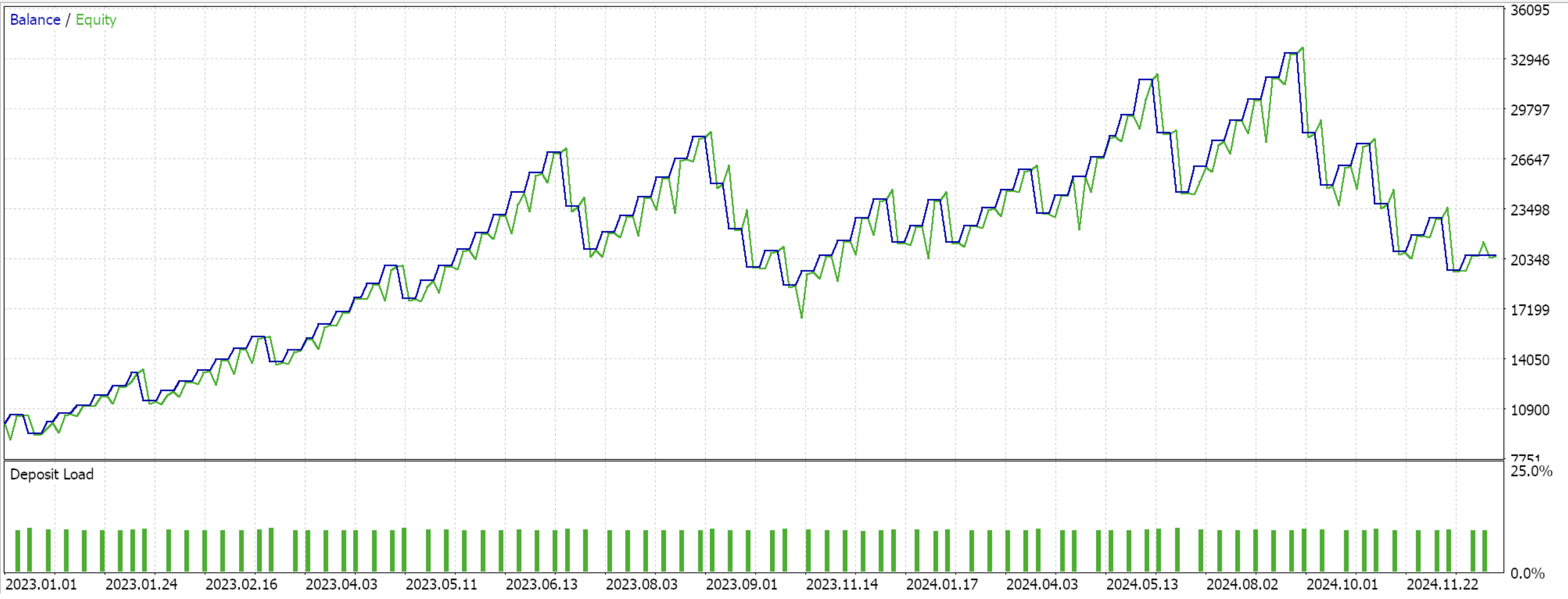
Post training and optimization, we perform test runs from 2023.01.01 to 2025.01.01, and we are presented by the following results for all 6 patterns/features:

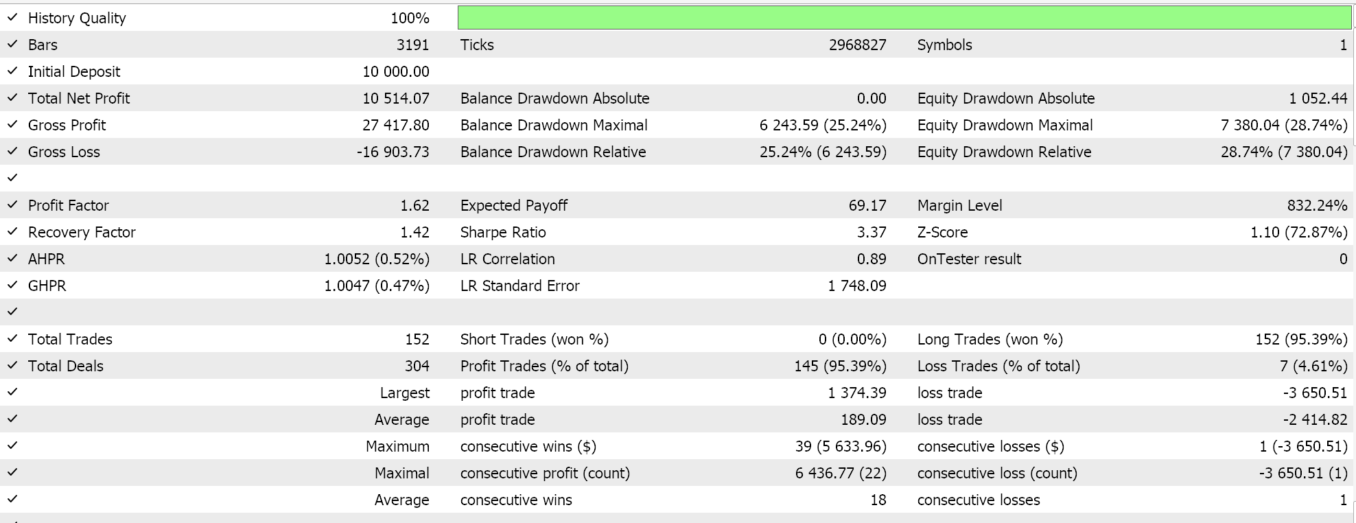
Feature 0 does not walk!

Feature 1 does not walk

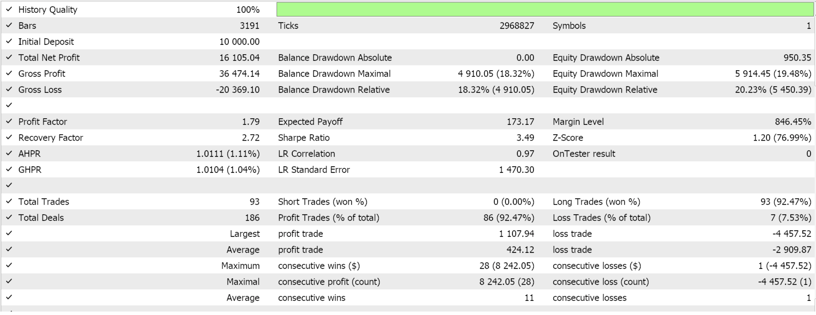
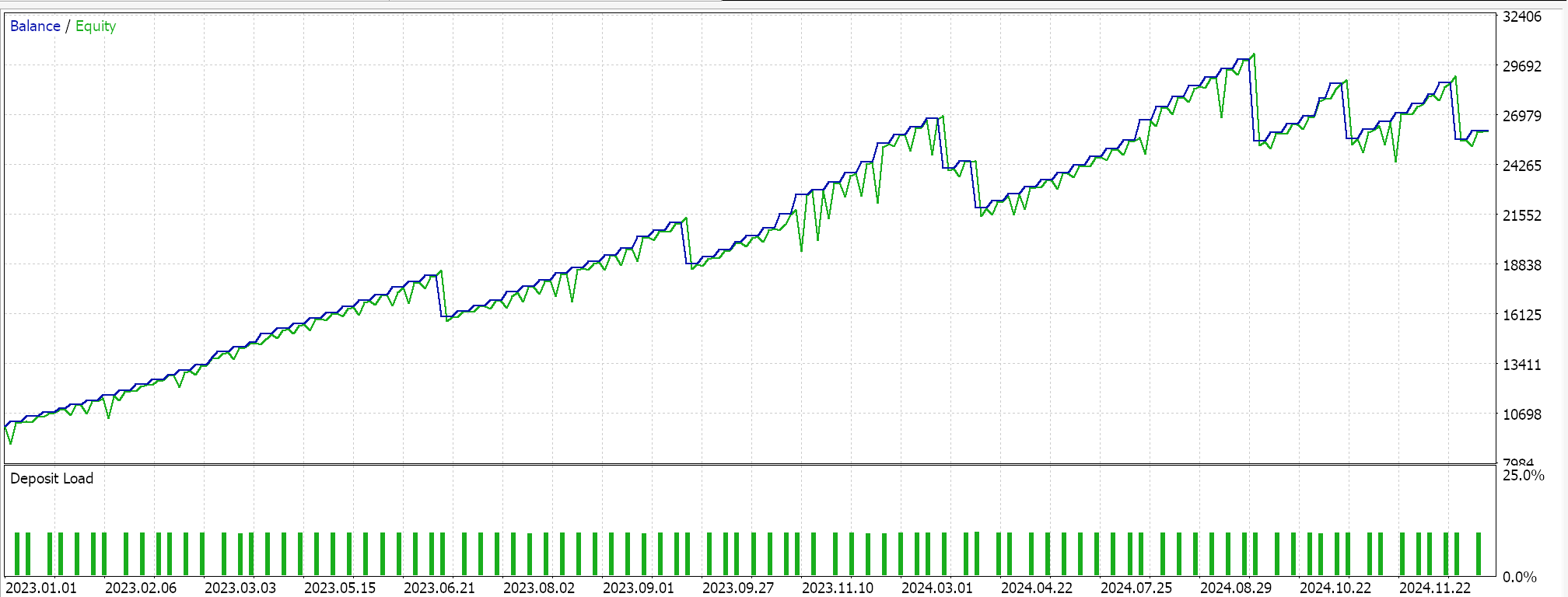
Feature 5 walks

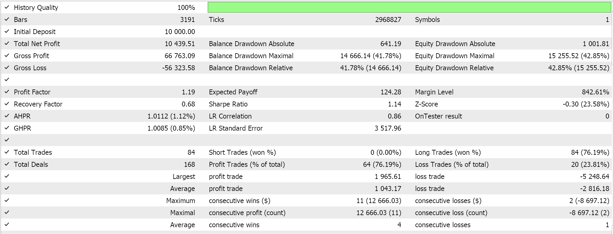
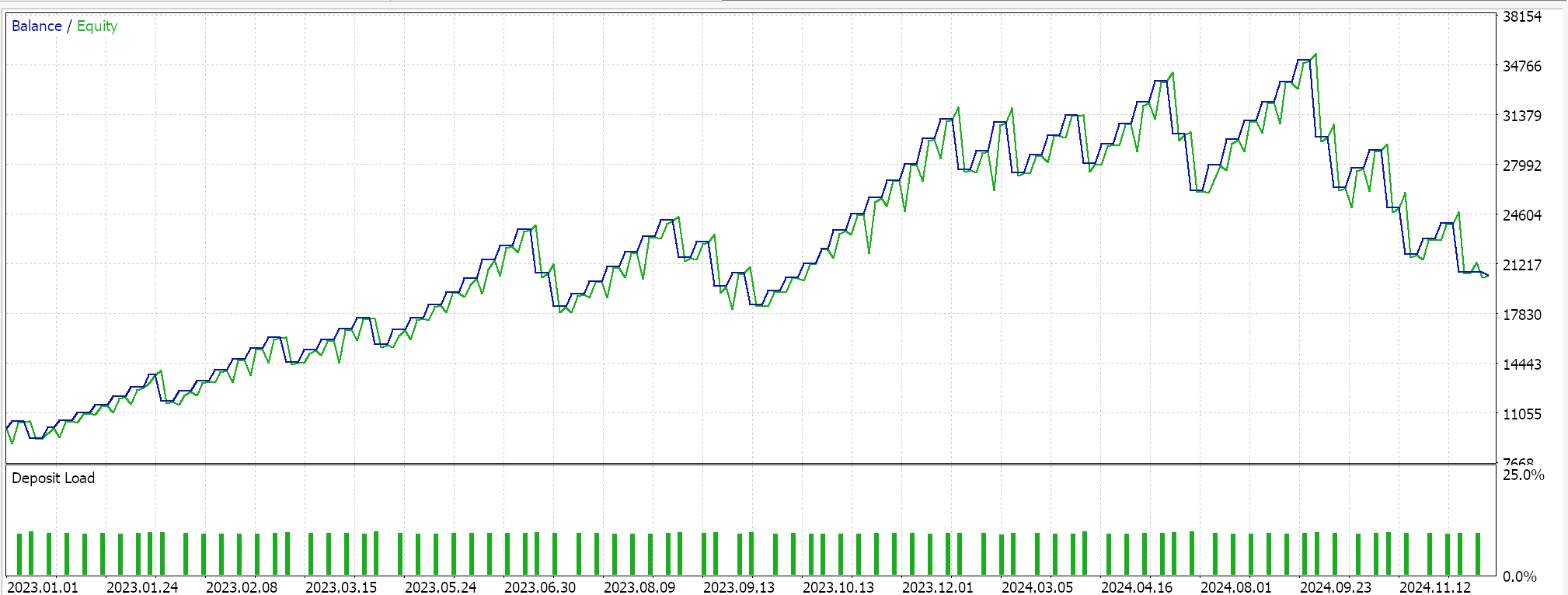
Feature 6 does not walk

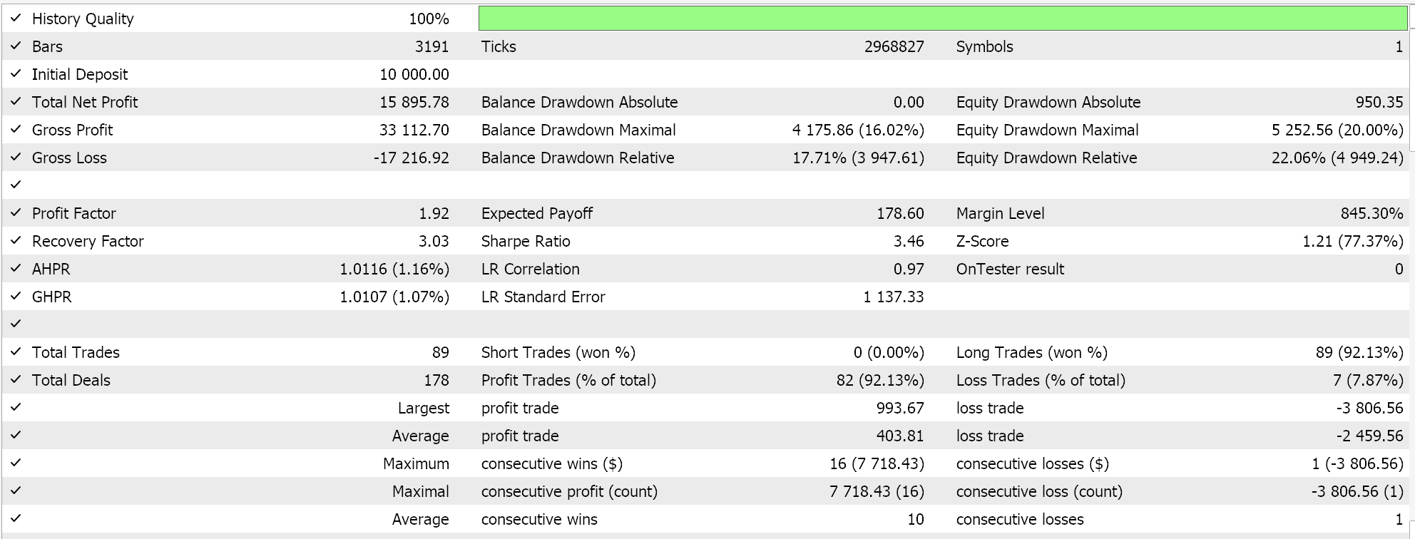
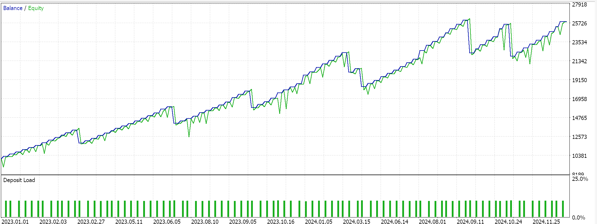
Feature 7 walks

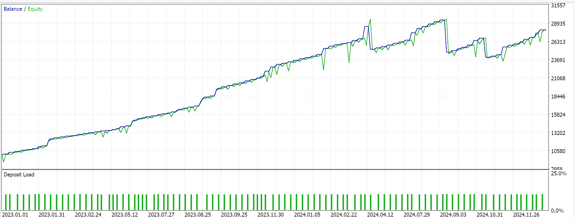
Feature 8 walks

Conclusion

We have examined patterns generated from combining the indicators of the DeMarker and the Envelopes. A momentum oscillator and a support/ resistance indicator, their complimentary pairing was first tested in the last article where trades were placed on a raw pattern basis. In this article, we processed these patterns through a recurrent neural network that uses the white noise kernel in training to process the same indicator patterns. We are yet to consider a neural network that brings together all patterns, something that was factitious with the raw signal patterns. We could look at this in coming articles.

Name	Description
wz64.mq5	Wizard Assembled Expert Advisor whose header shows files used
SignalWZ_64.mqh	Custom Signal Class file
64_0.onnx	Exported ONNX model for feature 0
64_1.onnx	Exported ONNX for feature 1
64_5.onnx	" for feature 5
64_6.onnx	" for feature 6
64_7.onnx	" for feature 7
64_8.onnx	' for feature 8